The ROBUSTREG Procedure

Example 98.4 Constructed Effects
The algorithms of PROC ROBUSTREG assume that a response variable is linearly dependent on the regressors. However, in practice, a response often depends on some factors in a nonlinear manner. This example demonstrates how a nonlinear response-factor relationship can be modeled by using constructed effects. (For more information, see the section EFFECT Statement in Chapter 19: Shared Concepts and Topics.)
The following data set contains 526 female observations and 474 male observations that are sampled from the 2003 National
Health and Nutrition Examination Survey (NHANES). Each observation is composed of three values, which correspond to the variables
BMI (body mass index), Age, and Gender, measured for subjects between ages 20 and 60.
data BMI;
   input BMI Age Gender $ @@;
   datalines;
46.16 30.33 F 20.67 31.83 F 30.98 51.33 F 30.71 31.42 F
29.81 30.50 M 19.94 25.08 F 29.97 41.67 F 24.48 26.92 F
34.34 51.25 F 20.24 53.67 F 27.72 60.25 F 32.85 41.67 M
22.75 47.50 F 32.78 22.42 F 43.07 29.50 F 38.34 58.50 F
40.03 39.92 F 21.78 56.42 M 28.77 39.83 F 28.77 28.75 F
29.73 54.25 M 33.75 35.67 M 28.48 35.83 M 22.12 29.58 F

   ... more lines ...

26.98 42.50 F 29.44 39.75 M 25.60 52.67 F 19.30 22.00 F
26.53 27.92 F 23.77 29.00 F 29.86 60.58 M 25.41 44.08 M
26.53 24.83 M 33.33 42.08 F 30.52 32.50 F 31.89 38.17 F
32.20 35.92 F 21.73 26.67 M 32.10 39.33 M 25.13 51.75 M
;
The goal of this analysis is to evaluate whether the BMI by Age curves for women and men are different at a 5% significance level. In order to provide sufficient flexibility to model the
effect of Age on BMI, you can use regression splines that you define by using an EFFECT statement. In this example, a regression spline of degree
2 that has three knots is used for the variable Age. The knots are placed at the 25th, 50th, and 75th percentiles of Age. This analysis assume that there is no interaction between Gender and Age, so that the BMI by Age curves for women and men are the same up to a constant. The following statements produce the BMI by Age scatter plot shown in Output 98.4.1:
proc sort data=bmi;
   by age;
run;

proc sgplot data=bmi;
   scatter x=age y=bmi/group=gender;
run;
Output 98.4.1: Scatter Plot for BMI Data
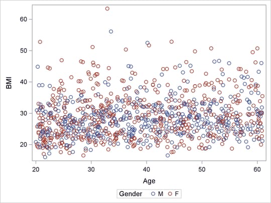
The observations that have large BMI values (for example, BMI > 40) are outliers that can substantially influence an ordinary least squares (OLS) analysis. Output 98.4.1 shows that the distributions of BMI conditional on Age are skewed toward the side of large BMI, and that there are more observations that have large BMI values (outliers) in the female group. Hence you can expect a significant Gender difference in the BMI by Age OLS regression analysis. This expectation is confirmed by the OLS Gender p-value 0.0059 in Output 98.4.2, which is produced by the following statements:
proc glmselect data=bmi;
   class gender;
   effect Age_Sp=spl(age/degree=2 knotmethod=percentiles(3));
   model bmi = gender age_sp /selection=none showpvalues;
   output out=out_ols P=pred R=res;
run;
Output 98.4.2: OLS Estimates
| Parameter Estimates | |||||
|---|---|---|---|---|---|
| Parameter | DF | Estimate | Standard Error |
t Value | Pr > |t| |
| Intercept | 1 | 29.890089 | 1.022825 | 29.22 | <.0001 |
| Gender F | 1 | 1.167332 | 0.422565 | 2.76 | 0.0058 |
| Gender M | 0 | 0 | . | . | . |
| Age_Sp 1 | 1 | -4.404487 | 1.473761 | -2.99 | 0.0029 |
| Age_Sp 2 | 1 | -3.329537 | 1.374096 | -2.42 | 0.0156 |
| Age_Sp 3 | 1 | -0.966875 | 1.314964 | -0.74 | 0.4623 |
| Age_Sp 4 | 1 | -1.611621 | 1.123854 | -1.43 | 0.1519 |
| Age_Sp 5 | 1 | -0.484787 | 1.701281 | -0.28 | 0.7757 |
| Age_Sp 6 | 0 | 0 | . | . | . |
A robust regression method can reduce the outlier influence by automatically assigning smaller or even zero weights to outliers.
For the BMI data, a robust regression method is likely to assign less weight to observations that have large BMI, so more
female observations than male observations would receive smaller weights. The following statements invoke PROC ROBUSTREG and
the BMI data set:
proc robustreg data=bmi method=s seed=100;
   class gender;
   effect Age_Sp=spl(age/degree=2 knotmethod=percentiles(3));
   model bmi = gender age_sp;
   output out=out_s P=pred R=res;
run;
Output 98.4.3 shows the parameter estimates and the diagnostics summary that are produced by PROC ROBUSTREG and the S method. In contrast
to OLS, the robust p-value 0.5581 of the Gender coefficient indicates that the Gender effect is not significant. The outlier diagnostics that are based on the S estimates find 19 outliers that are assigned lower
weights by the S method than by the OLS method.
Output 98.4.3: S Estimates and S Diagnostics Summary
| Parameter Estimates | ||||||||
|---|---|---|---|---|---|---|---|---|
| Parameter | DF | Estimate | Standard Error |
95% Confidence Limits | Chi-Square | Pr > ChiSq | ||
| Intercept | 1 | 28.2858 | 1.0081 | 26.3100 | 30.2616 | 787.33 | <.0001 | |
| Gender | F | 1 | 0.2409 | 0.4114 | -0.5654 | 1.0473 | 0.34 | 0.5581 |
| Gender | M | 0 | 0.0000 | . | . | . | . | . |
| Age_Sp | 1 | 1 | -3.8956 | 1.4376 | -6.7133 | -1.0779 | 7.34 | 0.0067 |
| Age_Sp | 2 | 1 | -1.8692 | 1.3430 | -4.5014 | 0.7630 | 1.94 | 0.1640 |
| Age_Sp | 3 | 1 | -0.8336 | 1.2877 | -3.3574 | 1.6903 | 0.42 | 0.5174 |
| Age_Sp | 4 | 1 | -0.2329 | 1.1055 | -2.3997 | 1.9338 | 0.04 | 0.8331 |
| Age_Sp | 5 | 1 | 0.0055 | 1.6632 | -3.2543 | 3.2652 | 0.00 | 0.9974 |
| Age_Sp | 6 | 0 | 0.0000 | . | . | . | . | . |
| Scale | 0 | 6.1715 | ||||||
To further compare the OLS and S outputs, the following statements plot the BMI predictions in the variable Age for both methods in the same graph, which is shown in Output 98.4.4:
data out2_s;
   set out_s;
   if gender="F" then label="F, S  ";
   if gender="M" then label="M, S  ";
run;

data out2_ols;
   merge bmi out_ols;
   if gender='F' then label='F, OLS';
   if gender='M' then label='M, OLS';
   keep pred bmi gender age label;
run;

data out2;
   set out2_ols out2_s;
run;

proc sgplot data=out2;
   series x=age y=pred/group=label;
run;
Output 98.4.4: OLS and S Predictions
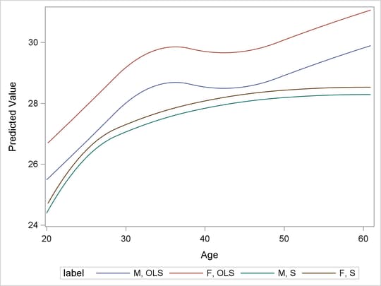
You can observe the following differences between the OLS and S predictions:
-
The OLS prediction is larger.
-
The OLS curves have a local maximum near
Age= 35.
One question remains: is the significance of the Gender effect for the OLS regression due solely to the outlying observations? To tentatively answer this question, the following
statements omit the observations that have the top 10% of BMI values from the original data set and reapply OLS and S methods to the reduced data set:
data three;
   set bmi;
   where bmi<38.315;
run;

proc robustreg data=three method=s seed=100;
   class gender;
   effect Age_Sp=spl(age/degree=2 knotmethod=percentiles(3));
   model bmi = gender age_sp;
   output out=out_s P=pred R=res;
run;
data out2_s;
   set out_s;
   if gender="F" then label="F, S  ";
   if gender="M" then label="M, S  ";
run;

proc glmselect data=three outdesign=four;
   class gender;
   effect Age_Sp=spl(age/degree=2 knotmethod=percentiles(3));
   model bmi = gender age_sp /selection=none showpvalues;
   output out=out_ols P=pred R=res;
run;
data out2_ols;
   merge three out_ols;
   if gender='F' then label='F, OLS';
   if gender='M' then label='M, OLS';
   keep pred bmi gender age label;
run;

data out2;
   set out2_ols out2_s;
run;

proc sgplot data=out2;
   series x=age y=pred/group=label;
run;
ods graphics off;
In the reduced data set, 71 female observations and 29 male observations are dropped. Output 98.4.5 and Output 98.4.6 show the refitted S and OLS parameter estimates, respectively.
Output 98.4.5: S Estimates
| Parameter Estimates | ||||||||
|---|---|---|---|---|---|---|---|---|
| Parameter | DF | Estimate | Standard Error |
95% Confidence Limits | Chi-Square | Pr > ChiSq | ||
| Intercept | 1 | 27.6427 | 0.9741 | 25.7334 | 29.5520 | 805.23 | <.0001 | |
| Gender | F | 1 | -0.2650 | 0.4023 | -1.0535 | 0.5234 | 0.43 | 0.5100 |
| Gender | M | 0 | 0.0000 | . | . | . | . | . |
| Age_Sp | 1 | 1 | -3.1859 | 1.4032 | -5.9361 | -0.4356 | 5.15 | 0.0232 |
| Age_Sp | 2 | 1 | -1.5354 | 1.3051 | -4.0934 | 1.0226 | 1.38 | 0.2394 |
| Age_Sp | 3 | 1 | -0.3776 | 1.2499 | -2.8273 | 2.0721 | 0.09 | 0.7626 |
| Age_Sp | 4 | 1 | 0.3299 | 1.0668 | -1.7610 | 2.4208 | 0.10 | 0.7572 |
| Age_Sp | 5 | 1 | 0.0949 | 1.6221 | -3.0845 | 3.2742 | 0.00 | 0.9534 |
| Age_Sp | 6 | 0 | 0.0000 | . | . | . | . | . |
| Scale | 0 | 4.9440 | ||||||
Output 98.4.6: OLS Estimates
| Parameter Estimates | |||||
|---|---|---|---|---|---|
| Parameter | DF | Estimate | Standard Error |
t Value | Pr > |t| |
| Intercept | 1 | 27.841568 | 0.780817 | 35.66 | <.0001 |
| Gender F | 1 | -0.040924 | 0.317749 | -0.13 | 0.8976 |
| Gender M | 0 | 0 | . | . | . |
| Age_Sp 1 | 1 | -3.253964 | 1.121292 | -2.90 | 0.0038 |
| Age_Sp 2 | 1 | -0.975273 | 1.034172 | -0.94 | 0.3459 |
| Age_Sp 3 | 1 | -0.508979 | 0.999609 | -0.51 | 0.6108 |
| Age_Sp 4 | 1 | 0.089393 | 0.852774 | 0.10 | 0.9165 |
| Age_Sp 5 | 1 | -0.113706 | 1.298157 | -0.09 | 0.9302 |
| Age_Sp 6 | 0 | 0 | . | . | . |
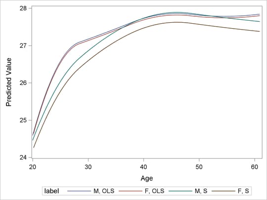
Output 98.4.7 displays the fitted curves on the reduced data set. You can see that Gender is no longer significant for the OLS model, and the OLS turning pattern has also disappeared, but the new S curves do not
change much from the previous ones. The OLS BMI by Age curves in Output 98.4.7 are closer to the S curves than to the OLS curves in Output 98.4.4. This suggests that the difference between the OLS and S estimate results is indeed due solely to the influence of the outlying
observations.
Output 98.4.7: OLS and S Predictions for the Reduced Data Set