The ROBUSTREG Procedure

Example 98.3 Growth Study of De Long and Summers
Robust regression and outlier detection techniques have considerable applications to econometrics. This example, from Zaman, Rousseeuw, and Orhan (2001), shows how these techniques substantially improve the ordinary least squares (OLS) results for the growth study of De Long and Summers.
De Long and Summers (1991) studied the national growth of 61 countries from 1960 to 1985 by applying OLS to the following data set:
data growth;
   input country $ GDP LFG EQP NEQ GAP @@;
   datalines;
Argentin  0.0089 0.0118 0.0214 0.2286 0.6079
Austria   0.0332 0.0014 0.0991 0.1349 0.5809
Belgium   0.0256 0.0061 0.0684 0.1653 0.4109
Bolivia   0.0124 0.0209 0.0167 0.1133 0.8634
Botswana  0.0676 0.0239 0.1310 0.1490 0.9474

   ... more lines ...

Venezuel  0.0120 0.0378 0.0340 0.0760 0.4974
Zambia   -0.0110 0.0275 0.0702 0.2012 0.8695
Zimbabwe  0.0110 0.0309 0.0843 0.1257 0.8875
;
The regression equation that they used is
![\[ \mr{GDP} = \beta _0 + \beta _1 \mr{LFG} + \beta _2 \mr{GAP} + \beta _3 \mr{EQP} + \beta _4 \mr{NEQ} +\epsilon \]](images/statug_rreg0276.png)
where the response variable is the growth in gross domestic product per worker (GDP) and the regressors are labor force growth (LFG), relative GDP gap (GAP), equipment investment (EQP), and nonequipment investment (NEQ).
The following statements invoke the REG procedure (see Chapter 97: The REG Procedure) for the OLS analysis:
proc reg data=growth;
   model GDP  = LFG GAP EQP NEQ;
run;
The OLS analysis that is shown in Output 98.3.1 indicates that GAP and EQP have a significant influence on GDP at the 5% level.
Output 98.3.1: OLS Estimates
| Parameter Estimates | |||||
|---|---|---|---|---|---|
| Variable | DF | Parameter Estimate |
Standard Error |
t Value | Pr > |t| |
| Intercept | 1 | -0.01430 | 0.01028 | -1.39 | 0.1697 |
| LFG | 1 | -0.02981 | 0.19838 | -0.15 | 0.8811 |
| GAP | 1 | 0.02026 | 0.00917 | 2.21 | 0.0313 |
| EQP | 1 | 0.26538 | 0.06529 | 4.06 | 0.0002 |
| NEQ | 1 | 0.06236 | 0.03482 | 1.79 | 0.0787 |
The following statements invoke the ROBUSTREG procedure and use the default M estimation:
ods graphics on;

proc robustreg data=growth plots=all;
   model GDP  = LFG GAP EQP NEQ / diagnostics leverage;
   id country;
run;

ods graphics off;
Output 98.3.2 displays model information and summary statistics for variables in the model.
Output 98.3.2: Model-Fitting Information and Summary Statistics
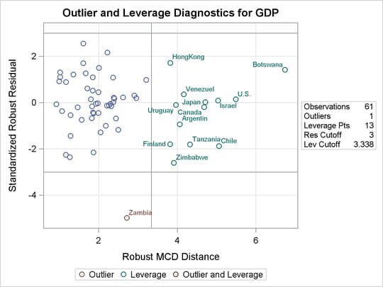
Output 98.3.3 displays the M estimates. Besides GAP and EQP, the robust analysis also indicates that NEQ is significant. This new finding is explained by Output 98.3.4, which shows that Zambia, the 60th country in the data, is an outlier. Output 98.3.4 also identifies leverage points that are based on the robust MCD distances; however, there are no serious high-leverage points in this data set.
Output 98.3.3: M Estimates
| Parameter Estimates | |||||||
|---|---|---|---|---|---|---|---|
| Parameter | DF | Estimate | Standard Error |
95% Confidence Limits | Chi-Square | Pr > ChiSq | |
| Intercept | 1 | -0.0247 | 0.0097 | -0.0437 | -0.0058 | 6.53 | 0.0106 |
| LFG | 1 | 0.1040 | 0.1867 | -0.2619 | 0.4699 | 0.31 | 0.5775 |
| GAP | 1 | 0.0250 | 0.0086 | 0.0080 | 0.0419 | 8.36 | 0.0038 |
| EQP | 1 | 0.2968 | 0.0614 | 0.1764 | 0.4172 | 23.33 | <.0001 |
| NEQ | 1 | 0.0885 | 0.0328 | 0.0242 | 0.1527 | 7.29 | 0.0069 |
| Scale | 1 | 0.0099 | |||||
Output 98.3.4: Diagnostics
| Diagnostics | ||||||
|---|---|---|---|---|---|---|
| Obs | country | Mahalanobis Distance | Robust MCD Distance | Leverage | Standardized Robust Residual |
Outlier |
| 1 | Argentin | 2.6083 | 4.0639 | * | -0.9424 | |
| 5 | Botswana | 3.4351 | 6.7391 | * | 1.4200 | |
| 8 | Canada | 3.1876 | 4.6843 | * | -0.1972 | |
| 9 | Chile | 3.6752 | 5.0599 | * | -1.8784 | |
| 17 | Finland | 2.6024 | 3.8186 | * | -1.7971 | |
| 23 | HongKong | 2.1225 | 3.8238 | * | 1.7161 | |
| 27 | Israel | 2.6461 | 5.0336 | * | 0.0909 | |
| 31 | Japan | 2.9179 | 4.7140 | * | 0.0216 | |
| 53 | Tanzania | 2.2600 | 4.3193 | * | -1.8082 | |
| 57 | U.S. | 3.8701 | 5.4874 | * | 0.1448 | |
| 58 | Uruguay | 2.5953 | 3.9671 | * | -0.0978 | |
| 59 | Venezuel | 2.9239 | 4.1663 | * | 0.3573 | |
| 60 | Zambia | 1.8562 | 2.7135 | -4.9798 | * | |
| 61 | Zimbabwe | 1.9634 | 3.9128 | * | -2.5959 | |
Output 98.3.5 displays robust versions of goodness-of-fit statistics for the model.
Output 98.3.5: Goodness-of-Fit Statistics
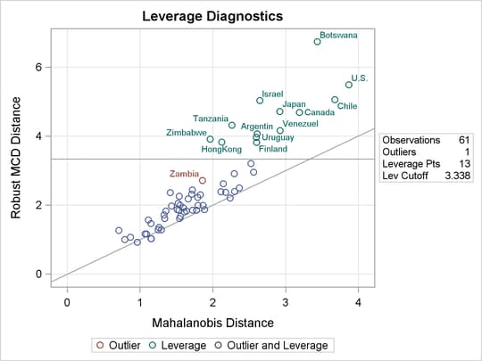
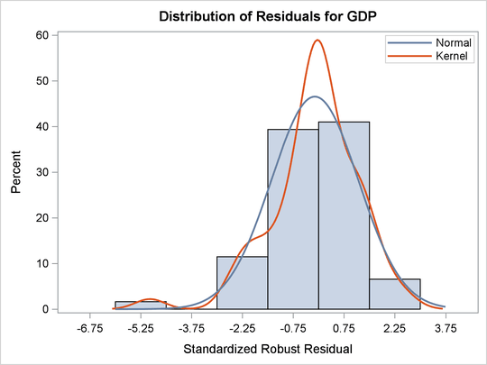
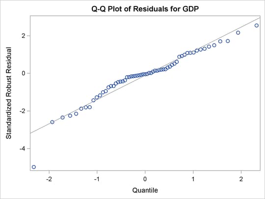
The PLOTS=ALL option generates four diagnostic plots. Output 98.3.6 and Output 98.3.7 are for outlier and leverage-point diagnostics. Output 98.3.8 and Output 98.3.9 are a histogram and a Q-Q plot, respectively, of the standardized robust residuals.
Output 98.3.6: RD Plot for Growth Data
Output 98.3.7: DD Plot for Growth Data
Output 98.3.8: Histogram
Output 98.3.9: Q-Q Plot
The following statements invoke the ROBUSTREG procedure and use LTS estimation, which was used by Zaman, Rousseeuw, and Orhan (2001). The results are consistent with those of M estimation.
proc robustreg method=lts(h=33) fwls data=growth seed=100;
   model GDP  = LFG GAP EQP NEQ / diagnostics leverage;
   id country;
run;
Output 98.3.10 displays the LTS estimates and the LTS R square.
Output 98.3.10: LTS Estimates and LTS R Square
Output 98.3.11 displays outlier and leverage-point diagnostics that are based on the LTS estimates and the robust MCD distances.
Output 98.3.11: Diagnostics
| Diagnostics | ||||||
|---|---|---|---|---|---|---|
| Obs | country | Mahalanobis Distance | Robust MCD Distance | Leverage | Standardized Robust Residual |
Outlier |
| 1 | Argentin | 2.6083 | 4.0639 | * | -1.0715 | |
| 5 | Botswana | 3.4351 | 6.7391 | * | 1.6574 | |
| 8 | Canada | 3.1876 | 4.6843 | * | -0.2324 | |
| 9 | Chile | 3.6752 | 5.0599 | * | -2.0896 | |
| 17 | Finland | 2.6024 | 3.8186 | * | -1.6367 | |
| 23 | HongKong | 2.1225 | 3.8238 | * | 1.7570 | |
| 27 | Israel | 2.6461 | 5.0336 | * | 0.2334 | |
| 31 | Japan | 2.9179 | 4.7140 | * | 0.0971 | |
| 53 | Tanzania | 2.2600 | 4.3193 | * | -1.2978 | |
| 57 | U.S. | 3.8701 | 5.4874 | * | 0.0605 | |
| 58 | Uruguay | 2.5953 | 3.9671 | * | -0.0857 | |
| 59 | Venezuel | 2.9239 | 4.1663 | * | 0.4113 | |
| 60 | Zambia | 1.8562 | 2.7135 | -4.4984 | * | |
| 61 | Zimbabwe | 1.9634 | 3.9128 | * | -2.1201 | |
Output 98.3.12 displays the final weighted least squares estimates, which are identical to those that are reported in Zaman, Rousseeuw, and Orhan (2001).
Output 98.3.12: Final Weighted LS Estimates
| Parameter Estimates for Final Weighted Least Squares Fit | |||||||
|---|---|---|---|---|---|---|---|
| Parameter | DF | Estimate | Standard Error |
95% Confidence Limits | Chi-Square | Pr > ChiSq | |
| Intercept | 1 | -0.0222 | 0.0093 | -0.0405 | -0.0039 | 5.65 | 0.0175 |
| LFG | 1 | 0.0446 | 0.1771 | -0.3026 | 0.3917 | 0.06 | 0.8013 |
| GAP | 1 | 0.0245 | 0.0082 | 0.0084 | 0.0406 | 8.89 | 0.0029 |
| EQP | 1 | 0.2824 | 0.0581 | 0.1685 | 0.3964 | 23.60 | <.0001 |
| NEQ | 1 | 0.0849 | 0.0314 | 0.0233 | 0.1465 | 7.30 | 0.0069 |
| Scale | 0 | 0.0116 | |||||