The QUANTREG Procedure

Optimization Algorithms
The optimization problem for median regression has been formulated and solved as a linear programming (LP) problem since the 1950s. Variations of the simplex algorithm, especially the method of Barrodale and Roberts (1973), have been widely used to solve this problem. The simplex algorithm is computationally demanding in large statistical applications, and in theory the number of iterations can increase exponentially with the sample size. This algorithm is often useful with data that contain no more than tens of thousands of observations.
Several alternatives have been developed to handle  regression for larger data sets. The interior point approach of Karmarkar (1984) solves a sequence of quadratic problems in which the relevant interior of the constraint set is approximated by an ellipsoid.
The worst-case performance of the interior point algorithm has been proved to be better than the worst-case performance of
the simplex algorithm. More important, experience has shown that the interior point algorithm is advantageous for larger problems.
regression for larger data sets. The interior point approach of Karmarkar (1984) solves a sequence of quadratic problems in which the relevant interior of the constraint set is approximated by an ellipsoid.
The worst-case performance of the interior point algorithm has been proved to be better than the worst-case performance of
the simplex algorithm. More important, experience has shown that the interior point algorithm is advantageous for larger problems.
Like regression, general quantile regression fits nicely into the standard primal-dual formulations of linear programming.
In addition to the interior point method, various heuristic approaches are available for computing -type solutions. Among these, the finite smoothing algorithm of Madsen and Nielsen (1993) is the most useful. It approximates the -type objective function with a smoothing function, so that the Newton-Raphson algorithm can be used iteratively to obtain
a solution after a finite number of iterations. The smoothing algorithm extends naturally to general quantile regression.
The QUANTREG procedure implements the simplex, interior point, and smoothing algorithms. The remainder of this section describes these algorithms in more detail.
Simplex Algorithm
Let ![$\bm {\mu } = [\mb{y}-\bA ^{\prime }\bbeta ]_+$](images/statug_qreg0076.png) ,
, ![$\bm {\nu } = [\bA ^{\prime }\bbeta -\mb{y}]_+$](images/statug_qreg0077.png) ,
, ![$\bm {\phi }=[\bbeta ]_+$](images/statug_qreg0078.png) , and
, and ![$\bm {\varphi }=[-\bbeta ]_+$](images/statug_qreg0079.png) , where
, where ![$[z]_+$](images/statug_qreg0080.png) is the nonnegative part of z.
is the nonnegative part of z.
Let 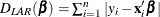 . For the problem, the simplex approach solves
  by reformulating it as the constrained minimization problem
![\[ \min _{\bbeta } \{ \mb{e}^{\prime } \bm {\mu } + \mb{e}^{\prime } \bm {\nu } | \mb{y} = \bA ^{\prime }\bbeta + \bm {\mu } - \bm {\nu }, \{ \bm {\mu }, \bm {\nu }\} \in \mb{R}_{+}^{n} \} \]](images/statug_qreg0083.png)
where  denotes an
  vector of ones.
Let ![$\bB =[ \bA ^{\prime }\ -\bA ^{\prime }\ \bI \ -\bI ]$](images/statug_qreg0085.png) ,
,  , and
, and  , where
  . The reformulation presents a standard LP problem:
This problem has the following dual formulation:
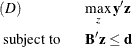
This formulation can be simplified as
![\[ \max _{z} \mb{y}^{\prime } \mb{z} ; \ \ \mbox{subject to } \bA \mb{z} = \mb{0}, \mb{z} \in [-1, 1]^ n \]](images/statug_qreg0091.png)
By setting 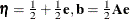 , the problem becomes
![\[ \max _{\bm {\eta }} \mb{y}^{\prime }\bm {\eta }; \ \ \mbox{subject to } \bA \bm {\eta } = \mb{b}, \bm {\eta } \in [0, 1]^ n \]](images/statug_qreg0093.png)
For quantile regression, the minimization problem is 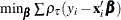 , and a similar set of steps leads to the dual formulation
![\[ \max _{z} \mb{y}^{\prime }\mb{z}; \ \ \mbox{subject to } \bA \mb{z} = (1-\tau ) \bA \mb{e}, \mb{z} \in [0, 1]^ n \]](images/statug_qreg0095.png)
The QUANTREG procedure solves this LP problem by using the simplex algorithm of Barrodale and Roberts (1973). This algorithm exploits the special structure of the coefficient matrix  by solving the primary LP problem (P) in two stages: The first stage chooses the columns in
  or
or  as pivotal columns. The second stage interchanges the columns in
  or – as basis or nonbasis columns, respectively. The algorithm obtains an optimal solution by executing these two stages interactively.
Moreover, because of the special structure of , only the main data matrix
or – as basis or nonbasis columns, respectively. The algorithm obtains an optimal solution by executing these two stages interactively.
Moreover, because of the special structure of , only the main data matrix  is stored in the current memory.
Although this special version of the simplex algorithm was introduced for median regression, it extends naturally to quantile regression for any given quantile and even to the entire quantile process (Koenker and d’Orey 1994). It greatly reduces the computing time that is required by the general simplex algorithm, and it is suitable for data sets with fewer than 5,000 observations and 50 variables.
Interior Point Algorithm
The ALGORITHM=INTERIOR option implements an interior point algorithm. This algorithm uses the primal-dual predictor-corrector method that is proposed by Lustig, Marsten, and Shanno (1992). Roos, Terlaky, and Vial (1997) provide more information about this particular algorithm. The following brief introduction of this algorithm uses the notation in the first reference.
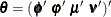
To be consistent with the conventional linear programming setting, let  , let
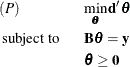
, let  , and let u be the general upper bound. The dual form of quantile regression solves the following linear programming primal problem:
-

-
subject to
-

-

This primal problem has n variables. The index i denotes a variable number, and k denotes an iteration number. If k is used as a subscript or superscript, it denotes "of iteration k."
Let  be the primal slack so that
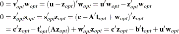
  . Associate dual variables w with these constraints. The interior point algorithm solves the system of equations to satisfy the Karush-Kuhn-Tucker (KKT)
conditions for optimality:
. Associate dual variables w with these constraints. The interior point algorithm solves the system of equations to satisfy the Karush-Kuhn-Tucker (KKT)
conditions for optimality:
These are the conditions for feasibility, with the addition of complementarity conditions  and
and  .
The equality
.
The equality  must occur at the optimum. Complementarity forces the optimal objectives of the primal and dual to be equal,
 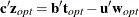 , because
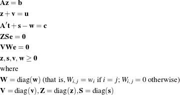
Therefore
![\[ 0 = \mb{c}^{\prime } \mb{z}_{\mathit{opt}} - \mb{b}^{\prime } \mb{t}_{\mathit{opt}} + \mb{u}^{\prime } \mb{w}_{\mathit{opt}} \]](images/statug_qreg0114.png)
The duality gap,  , measures the convergence of the algorithm. You can specify a tolerance for this convergence criterion in the TOLERANCE=
option in the PROC QUANTREG statement.
, measures the convergence of the algorithm. You can specify a tolerance for this convergence criterion in the TOLERANCE=
option in the PROC QUANTREG statement.
Before the optimum is reached, it is possible for a solution  to violate the KKT conditions in one of several ways:
-
Primal bound constraints can be broken:
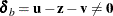 .
.
-
Primal constraints can be broken:
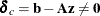 .
.
-
Dual constraints can be broken:
 .
.
-
Complementarity conditions are unsatisfied:
 and
and  .
.
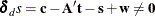
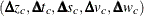
The interior point algorithm works by using Newton’s method to find a direction  to move from the current solution
  toward a better solution:
![\[ (\mb{z}^{k+1}, \mb{t}^{k+1}, \mb{s}^{k+1}, \mb{v}^{k+1}, \mb{w}^{k+1}) = (\mb{z}^ k, \mb{t}^ k, \mb{s}^ k, \mb{v}^ k, \mb{w}^ k) + \kappa (\bDelta z^ k, \bDelta t^ k, \bDelta s^ k, \bDelta v^ k, \bDelta w^ k) \]](images/statug_qreg0124.png)
 is the step length and is assigned a value as large as possible, but not so large that a
  or
or  is "too close" to 0. You can control the step length in the KAPPA= option in the PROC QUANTREG statement.
The QUANTREG procedure implements a predictor-corrector variant of the primal-dual interior point algorithm.
First, Newton’s method is used to find a direction 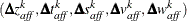 in which to move. This is known as the affine step.
In iteration k, the affine step system that must be solved is
Therefore, the following computations are involved in solving the affine step, where is the step length as before:

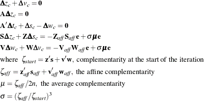
The success of the affine step is gauged by calculating the complementarity of  and
and  at
at 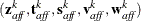 and comparing it with the complementarity at the starting point . If the affine step was successful in reducing the complementarity by a substantial amount, the need for centering is not
great. Therefore, a value close to 0 is assigned to
and comparing it with the complementarity at the starting point . If the affine step was successful in reducing the complementarity by a substantial amount, the need for centering is not
great. Therefore, a value close to 0 is assigned to  in the following second linear system, which is used to determine a centering vector.
The following linear system is solved to determine a centering vector
 from
from 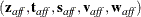 :
:
However, if the affine step was unsuccessful, then centering is deemed beneficial, and a value close to 1.0 is assigned to
. In other words, the value of is adaptively altered depending on the progress made toward the optimum.
Therefore, the following computations are involved in solving the centering step:
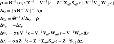
Then

where, as before, is the step length, which is assigned a value as large as possible but not so large that a , ,  , or
, or  is "too close" to 0.
Although the predictor-corrector variant entails solving two linear systems instead of one, fewer iterations are usually required
to reach the optimum. The additional overhead of the second linear system is small because the matrix  has already been factorized in order to solve the first linear system.
You can specify the starting point in the INEST= option in the PROC QUANTREG statement. By default, the starting point is set to be the least squares estimate.
Efficient Interior Point Algorithm
The ALGORITHM=IPM option implements a more efficient interior point algorithm than the one that is used when ALGORITHM=INTERIOR.
The computing strategy of the ALGORITHM=IPM option is the same as the strategy for the ALGORITHM=INTERIOR option, but the
ALGORITHM=IPM option implements the algorithm by using more efficient matrix functions. The ALGORITHM=IPM option uses the
complementarity value to measure the convergence of the algorithm, which is different from the dual gap value that is used
when ALGORITHM=INTERIOR. The complementarity value is defined as  . You can specify a tolerance for this complementarity convergence criterion by using the TOLERANCE= option in the PROC QUANTREG
statement. Unlike the ALGORITHM=INTERIOR option, the ALGORITHM=IPM option does not support the KAPPA= option.
. You can specify a tolerance for this complementarity convergence criterion by using the TOLERANCE= option in the PROC QUANTREG
statement. Unlike the ALGORITHM=INTERIOR option, the ALGORITHM=IPM option does not support the KAPPA= option.
Smoothing Algorithm
To minimize the sum of the absolute residuals  , the smoothing algorithm approximates the nondifferentiable function
  by the following smooth function(which is referred to as the Huber function),
![\[ D_{\gamma }(\bbeta ) = \sum _{i=1}^ n H_{\gamma }(r_ i(\bbeta )) \]](images/statug_qreg0145.png)
where
![\[ H_{\gamma }(t) = \left\{ \begin{array}{ll} t^2 \slash (2\gamma ) & {\mbox{if }} |t| \leq \gamma \\ |t| - \gamma \slash 2 & {\mbox{if }} |t| > \gamma \end{array} \right. \]](images/statug_qreg0146.png)
Here  , and the threshold
  is a positive real number. The function
  is continuously differentiable, and a minimizer
  of is close to a minimizer
  of when is close to 0.
The advantage of the smoothing algorithm as described in Madsen and Nielsen (1993) is that the solution can be detected when  is small. In other words, it is not necessary to let converge to 0 in order to find a minimizer of . The algorithm terminates before going through the entire sequence of values of that are generated by the algorithm. Convergence is indicated by no change of the status of residuals
  as goes through this sequence.
The smoothing algorithm extends naturally from regression to general quantile regression (Chen 2007). The function
![\[ D_{\rho _\tau }(\bbeta ) = \sum _{i=1}^ n \rho _{\tau }(y_ i-\mb{x}_ i^{\prime }\bbeta ) \]](images/statug_qreg0154.png)
can be approximated by the smooth function
![\[ D_{\gamma ,\tau }(\bbeta ) = \sum _{i=1}^ n H_{\gamma ,\tau }(r_ i(\bbeta )) \]](images/statug_qreg0155.png)
where
![\[ H_{\gamma ,\tau }(t) = \left\{ \begin{array}{lll} t(\tau -1)-{\frac12}(\tau -1)^2\gamma & {\mbox{if }} t\le (\tau -1)\gamma \\ {\frac{t^2}{2\gamma }} & {\mbox{if }} (\tau -1)\gamma \leq t \leq \tau \gamma \\ t\tau - {\frac12}\tau ^2\gamma & {\mbox{if }} t\ge \tau \gamma \end{array} \right. \]](images/statug_qreg0156.png)
The function  is determined by whether
 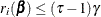 ,
,  , or
, or 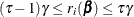 . These inequalities divide
  into subregions that are separated by the parallel hyperplanes
 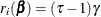 and
and  . The set of all such hyperplanes is denoted by
  :
:
![\[ B_{\gamma , \tau } = \{ \bbeta \in \mb{R}^ p | \exists i: r_ i(\bbeta )=(\tau -1)\gamma \mbox{ or } r_ i(\bbeta )=\tau \gamma \} \]](images/statug_qreg0165.png)
Define the sign vector  as
as
![\[ s_ i = s_ i(\bbeta ) = \left\{ \begin{array}{rl} -1 & {\mbox{if }} r_ i(\bbeta )\le (\tau -1)\gamma \\ 0 & {\mbox{if }} (\tau -1)\gamma \leq r_ i(\bbeta ) \leq \tau \gamma \\ 1 & {\mbox{if }} r_ i(\bbeta )\ge \tau \gamma \end{array} \right. \]](images/statug_qreg0167.png)
and introduce
![\[ w_ i = w_ i(\bbeta ) = 1- s_ i^2(\bbeta ) \]](images/statug_qreg0168.png)
Therefore,
![\begin{eqnarray*} & & H_{\gamma ,\tau }(r_ i(\bbeta )) = {\frac1{2\gamma }} w_ i r_ i^2(\bbeta ) \\ & & + s_ i [ {\frac12} r_ i(\bbeta ) + {\frac14}(1-2\tau )\gamma + s_ i( r_ i(\bbeta )(\tau -{\frac12}) - {\frac14}( 1 - 2\tau + 2\tau ^2)\gamma )] \end{eqnarray*}](images/statug_qreg0169.png)
This equation yields
![\[ D_{\gamma ,\tau }(\bbeta ) = {\frac1{2\gamma }} \mb{r}^{\prime }\bW _{\gamma ,\tau } \mb{r} + \mb{v}^{\prime }(s) \mb{r} + c(s) \]](images/statug_qreg0170.png)
where  is the diagonal
  matrix with diagonal elements
  ,
,  ,
, ![$c(s) = \sum [ {\frac14} (1-2\tau )\gamma s_ i - {\frac14} s_ i^2 ( 1-2\tau + 2\tau ^2 ) \gamma ]$](images/statug_qreg0175.png) , and
, and  .
.
The gradient of  is given by
![\[ D^{(1)}_{\gamma , \tau }(\bbeta ) = -\bA [ {\frac1\gamma } \bW _{\gamma ,\tau }(\bbeta ) r(\bbeta ) + v(s)] \]](images/statug_qreg0178.png)
For  the Hessian exists and is given by
![\[ D^{(2)}_{\gamma ,\tau }(\bbeta ) = {\frac1\gamma }\bA \bW _{\gamma ,\tau }(\bbeta ) \bA ^{\prime } \]](images/statug_qreg0180.png)
The gradient is a continuous function in , whereas the Hessian is piecewise constant.
Following Madsen and Nielsen (1993), the vector  is referred to as a -feasible sign vector if there exists with
  . If is -feasible, then
  is defined as the quadratic function
  that is derived from
  by substituting for
  . Thus, for any
  with
with  ,
,
![\[ Q_ s(\balpha ) = {\frac12}(\balpha -\bbeta )^{\prime } D^{(2)}_{\gamma ,\tau }(\bbeta ) (\balpha -\bbeta ) + D^{(1)}_{\gamma ,\tau }(\bbeta ) (\balpha -\bbeta ) + D_{\gamma ,\tau }(\bbeta ) \]](images/statug_qreg0189.png)
In the domain  ,
,
![\[ D_{\gamma ,\tau }(\alpha ) = Q_ s(\balpha ) \]](images/statug_qreg0191.png)
For each and  , there can be one or several corresponding quadratics, . If
  , then is characterized by
  and . However, for
  , the quadratic is not unique. Therefore, the following reference determines the quadratic:
![\[ (\gamma , \theta , \mb{s}) \]](images/statug_qreg0196.png)
Again following Madsen and Nielsen (1993), let  be a feasible reference if is a -feasible sign vector, where
  , and let be a solution reference if is feasible and minimizes .
The smoothing algorithm for minimizing  is based on minimizing for a set of decreasing . For each new value of , information from the previous solution is used. Finally, when is small enough, a solution can be found by the following modified Newton-Raphson algorithm as stated by Madsen and Nielsen
(1993):
is based on minimizing for a set of decreasing . For each new value of , information from the previous solution is used. Finally, when is small enough, a solution can be found by the following modified Newton-Raphson algorithm as stated by Madsen and Nielsen
(1993):
-
Find an initial solution reference
 .
.
-
Repeat the following substeps until
 .
.
-
Decrease
.
-
Find a solution reference
 .
.
 is the solution.
-
By default, the initial solution reference is found by letting  be the least squares solution. Alternatively, you can specify the initial solution reference with the INEST= option in the
PROC QUANTREG statement. Then and are chosen according to these initial values.
be the least squares solution. Alternatively, you can specify the initial solution reference with the INEST= option in the
PROC QUANTREG statement. Then and are chosen according to these initial values.
There are several approaches for determining a decreasing sequence of values of . The QUANTREG procedure uses a strategy by Madsen and Nielsen (1993). The computation that is uses is not significant compared to the Newton-Raphson step. You can control the ratio of consecutive
decreasing values of by specifying the RRATIO= suboption in the ALGORITHM= option in the PROC QUANTREG statement. By default,
![\[ {\mbox{RRATIO }} = \left\{ \begin{array}{ll} 0.1 & {\mbox{ if }} n \ge 10,000 {\mbox{ and }} p\le 20 \\ 0.9 & {\mbox{ if }} {\frac pn} \ge 0.1 {\mbox{ or }} \left\{ n \le 5,000 {\mbox{ and }} p\ge 300 \right\} \\ 0.5 & {\mbox{ otherwise }} \end{array} \right. \]](images/statug_qreg0205.png)
For the and quantile regression, it turns out that the smoothing algorithm is very efficient and competitive, especially for a fat data set—namely, when  and
and  is dense. See Chen (2007) for a complete smoothing algorithm and details.