The KDE Procedure

Convolutions
The formulas for the binned estimator  in the previous subsection are in the form of a convolution product between two matrices, one of which contains the bin counts,
the other of which contains the rescaled kernels evaluated at multiples of grid increments. This section defines these two
matrices explicitly, and shows that is their convolution.
in the previous subsection are in the form of a convolution product between two matrices, one of which contains the bin counts,
the other of which contains the rescaled kernels evaluated at multiples of grid increments. This section defines these two
matrices explicitly, and shows that is their convolution.
Beginning with the weighted univariate case, define the following matrices:
The first thing to note is that many terms in  are negligible. The term
  is taken to be 0 when
  , so you can define
![\[ l = \min (g-1,\mr{floor}(5h/\delta )) \]](images/statug_kde0068.png)
as the maximum integer multiple of the grid increment to get nonzero evaluations of the rescaled kernel. Here  denotes the largest integer less than or equal to x.
Next, let p be the smallest power of 2 that is greater than  ,
,
![\[ p = 2^{\mr{ceil}(\log _{2} (g+l+1))} \]](images/statug_kde0071.png)
where  denotes the smallest integer greater than or equal to x.
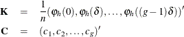
Modify as follows:
![\[ \bK = \frac{1}{n}(\varphi _{h}(0), \varphi _{h}(\delta ), \ldots ,\varphi _{h}(l\delta ), \underbrace{0,\ldots ,0}_{p-2l-1}, \varphi _{h}(l\delta ), \ldots ,\varphi _{h}(\delta ))’ \]](images/statug_kde0073.png)
Essentially, the negligible terms of are omitted, and the rest are symmetrized (except for one term). The whole matrix is then padded to size  with zeros in the middle. The dimension p is a highly composite number—that is, one that decomposes into many factors—leading to the most efficient fast Fourier transform
operation (see Wand; 1994).
with zeros in the middle. The dimension p is a highly composite number—that is, one that decomposes into many factors—leading to the most efficient fast Fourier transform
operation (see Wand; 1994).
The third operation is to pad the bin count matrix  with zeros to the same size as :
![\[ \bC = (c_{1},c_{2},\ldots ,c_{g}, \underbrace{0,\ldots ,0}_{p-g})’ \]](images/statug_kde0076.png)
The convolution  is then a matrix, and the preceding formulas show that its first g entries are exactly the estimates
 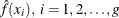 .
.
For bivariate smoothing, the matrix is defined similarly as
![\[ \bK = \left[ \begin{array}{cccccccccc}\kappa _{0,0} & \kappa _{0,1} & \ldots & \kappa _{0,l_{Y}} & \mb{0} & \kappa _{0,l_{Y}} & \ldots & \kappa _{0,1} \\ \kappa _{1,0} & \kappa _{1,1} & \ldots & \kappa _{1,l_{Y}} & \mb{0} & \kappa _{1,l_{Y}} & \ldots & \kappa _{1,1} \\ \vdots \\ \kappa _{l_{X},0} & \kappa _{l_{X},1} & \ldots & \kappa _{l_{X},l_{Y}} & \mb{0} & \kappa _{l_{X},l_{Y}} & \ldots & \kappa _{l_{X},1} \\ \mb{0} & \mb{0} & \ldots & \mb{0} & \mb{0} & \mb{0} & \ldots & \mb{0} \\ \kappa _{l_{X},0} & \kappa _{l_{X},1} & \ldots & \kappa _{l_{X},l_{Y}} & \mb{0} & \kappa _{l_{X},l_{Y}} & \ldots & \kappa _{l_{X},1} \\ \vdots \\ \kappa _{1,0} & \kappa _{1,1} & \ldots & \kappa _{1,l_{Y}} & \mb{0} & \kappa _{1,l_{Y}} & \ldots & \kappa _{1,1} \end{array} \right]_{p_{X} \times p_{Y}} \]](images/statug_kde0079.png)
where  , and so forth, and
  .
.
The bin count matrix is defined as
![\[ \bC = \left[ \begin{array}{ccccccc} {c}_{1,1} & {c}_{1,2} & \ldots & {c}_{1,g_{Y}} & 0 & \ldots & 0\\ {c}_{2,1} & {c}_{2,2} & \ldots & {c}_{2,g_{Y}} & 0 & \ldots & 0\\ \vdots \\ {c}_{g_{X},1} & {c}_{g_{X},2} & \ldots & {c}_{g_{X},g_{Y}} & 0 & \ldots & 0 \\ 0 & 0 & \ldots & 0 & 0 & \ldots & 0 \\ \vdots \\ 0 & 0 & \ldots & 0 & 0 & \ldots & 0 \end{array} \right]_{p_{X} \times p_{Y}} \]](images/statug_kde0082.png)
As with the univariate case, the  upper-left corner of the convolution is the matrix of the estimates
  .
.
Most of the results in this subsection are found in Wand (1994).