The FREQ Procedure

The FREQ procedure provides easy access to statistics for testing for association in a crosstabulation table.
In this example, high school students applied for courses in a summer enrichment program; these courses included journalism, art history, statistics, graphic arts, and computer programming. The students accepted were randomly assigned to classes with and without internships in local companies. Table 40.1 contains counts of the students who enrolled in the summer program by gender and whether they were assigned an internship slot.
Table 40.1: Summer Enrichment Data
|
Enrollment |
||||
|---|---|---|---|---|
|
Gender |
Internship |
Yes |
No |
Total |
|
boys |
yes |
35 |
29 |
64 |
|
boys |
no |
14 |
27 |
41 |
|
girls |
yes |
32 |
10 |
42 |
|
girls |
no |
53 |
23 |
76 |
The SAS data set SummerSchool is created by inputting the summer enrichment data as cell count data, or providing the frequency count for each combination
of variable values. The following DATA step statements create the SAS data set SummerSchool:
data SummerSchool;
   input Gender $ Internship $ Enrollment $ Count @@;
   datalines;
boys  yes yes 35   boys  yes no 29
boys   no yes 14   boys   no no 27
girls yes yes 32   girls yes no 10
girls  no yes 53   girls  no no 23
;
The variable Gender takes the values ‘boys’ or ‘girls,’ the variable Internship takes the values ‘yes’ and ‘no,’ and the variable Enrollment takes the values ‘yes’ and ‘no.’ The variable Count contains the number of students that correspond to each combination of data values. The double at sign (@@) indicates that
more than one observation is included on a single data line. In this DATA step, two observations are included on each line.
Researchers are interested in whether there is an association between internship status and summer program enrollment. The
Pearson chi-square statistic is an appropriate statistic to assess the association in the corresponding ![]() table. The following PROC FREQ statements specify this analysis.
table. The following PROC FREQ statements specify this analysis.
You specify the table for which you want to compute statistics with the TABLES statement. You specify the statistics you want to compute with options after a slash (/) in the TABLES statement.
proc freq data=SummerSchool order=data;
   tables Internship*Enrollment / chisq;
   weight Count;
run;
The ORDER= option controls the order in which variable values are displayed in the rows and columns of the table. By default, the values are arranged according to the alphanumeric order of their unformatted values. If you specify ORDER=DATA, the data are displayed in the same order as they occur in the input data set. Here, because ‘yes’ appears before ‘no’ in the data, ‘yes’ appears first in any table. Other options for controlling order include ORDER=FORMATTED, which orders according to the formatted values, and ORDER=FREQUENCY, which orders by descending frequency count.
In the TABLES statement, Internship*Enrollment specifies a table where the rows are internship status and the columns are program enrollment. The CHISQ option requests
chi-square statistics for assessing association between these two variables. Because the input data are in cell count form,
the WEIGHT statement is required. The WEIGHT statement names the variable Count, which provides the frequency of each combination of data values.
Figure 40.1 presents the crosstabulation of Internship and Enrollment. In each cell, the values printed under the cell count are the table percentage, row percentage, and column percentage, respectively.
For example, in the first cell, 63.21 percent of the students offered courses with internships accepted them and 36.79 percent
did not.
Figure 40.2 displays the statistics produced by the CHISQ option. The Pearson chi-square statistic is labeled 'Chi-Square' and has a value of 0.8189 with 1 degree of freedom. The associated p-value is 0.3655, which means that there is no significant evidence of an association between internship status and program enrollment. The other chi-square statistics have similar values and are asymptotically equivalent. The other statistics (phi coefficient, contingency coefficient, and Cramér’s V) are measures of association derived from the Pearson chi-square. For Fisher’s exact test, the two-sided p-value is 0.4122, which also shows no association between internship status and program enrollment.
The analysis, so far, has ignored gender. However, it might be of interest to ask whether program enrollment is associated with internship status after adjusting for gender. You can address this question by doing an analysis of a set of tables (in this case, by analyzing the set consisting of one for boys and one for girls). The Cochran-Mantel-Haenszel (CMH) statistic is appropriate for this situation: it addresses whether rows and columns are associated after controlling for the stratification variable. In this case, you would be stratifying by gender.
The PROC FREQ statements for this analysis are very similar to those for the first analysis, except that there is a third
variable, Gender, in the TABLES statement. When you cross more than two variables, the two rightmost variables construct the rows and columns
of the table, respectively, and the leftmost variables determine the stratification.
The following PROC FREQ statements also request frequency plots for the crosstabulation tables. PROC FREQ produces these plots by using ODS Graphics to create graphs as part of the procedure output. ODS Graphics must be enabled before producing plots. The PLOTS(ONLY)=FREQPLOT option requests frequency plots. The TWOWAY=CLUSTER plot-option specifies a cluster layout for the two-way frequency plots.
ods graphics on;
proc freq data=SummerSchool;
   tables Gender*Internship*Enrollment /
          chisq cmh plots(only)=freqplot(twoway=cluster);
   weight Count;
run;
ods graphics off;
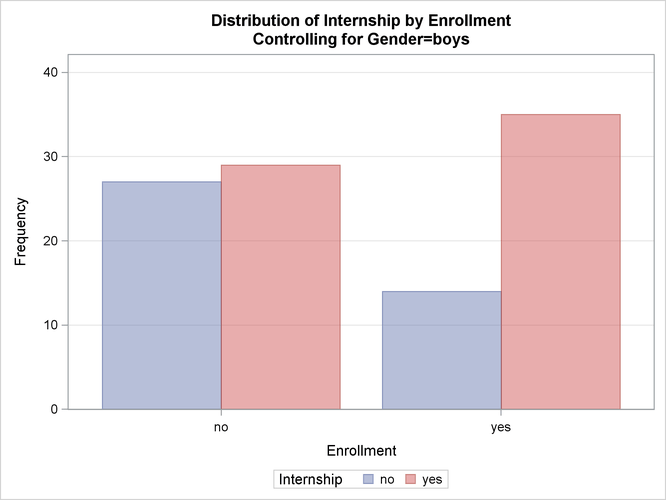
This execution of PROC FREQ first produces two individual crosstabulation tables of Internship by Enrollment: one for boys and one for girls. Frequency plots and chi-square statistics are produced for each individual table. Figure 40.3, Figure 40.4, and Figure 40.5 show the results for boys. Note that the chi-square statistic for boys is significant at the ![]() level of significance. Boys offered a course with an internship are more likely to enroll than boys who are not.
level of significance. Boys offered a course with an internship are more likely to enroll than boys who are not.
Figure 40.4 displays the frequency plot of Internship by Enrollment for boys. By default, frequency plots are displayed as bar charts. You can use PLOTS= options to request dot plots instead
of bar charts, to change the orientation of the bars from vertical to horizontal, and to change the scale from frequencies
to percents. You can also use PLOTS= options to specify other two-way layouts (stacked, vertical groups, or horizontal groups)
and to change the primary grouping from column levels to row levels.
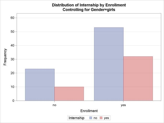
Figure 40.6, Figure 40.7, and Figure 40.8 display the crosstabulation table, frequency plot, and chi-square statistics for girls. You can see that there is no evidence of association between internship offers and program enrollment for girls.
These individual table results demonstrate the occasional problems with combining information into one table and not accounting
for information in other variables such as Gender. Figure 40.9 contains the CMH results. There are three summary (CMH) statistics; which one you use depends on whether your rows and/or
columns have an order in ![]() tables. However, in the case of
tables. However, in the case of ![]() tables, ordering does not matter and all three statistics take the same value. The CMH statistic follows the chi-square distribution
under the hypothesis of no association, and here, it takes the value 4.0186 with 1 degree of freedom. The associated p-value is 0.0450, which indicates a significant association at the
tables, ordering does not matter and all three statistics take the same value. The CMH statistic follows the chi-square distribution
under the hypothesis of no association, and here, it takes the value 4.0186 with 1 degree of freedom. The associated p-value is 0.0450, which indicates a significant association at the ![]() level.
level.
Thus, when you adjust for the effect of gender in these data, there is an association between internship and program enrollment.
But, if you ignore gender, no association is found. Note that the CMH option also produces other statistics, including estimates
and confidence limits for relative risk and odds ratios for ![]() tables and the Breslow-Day Test. These results are not displayed here.
tables and the Breslow-Day Test. These results are not displayed here.