The GENMOD Procedure
-
Overview

-
Getting Started
-
SyntaxPROC GENMOD StatementASSESS StatementBAYES StatementBY StatementCLASS StatementCODE StatementCONTRAST StatementDEVIANCE StatementEFFECTPLOT StatementESTIMATE StatementEXACT StatementEXACTOPTIONS StatementFREQ StatementFWDLINK StatementINVLINK StatementLSMEANS StatementLSMESTIMATE StatementMODEL StatementOUTPUT StatementProgramming StatementsREPEATED StatementSLICE StatementSTORE StatementSTRATA StatementVARIANCE StatementWEIGHT StatementZEROMODEL Statement
-
DetailsGeneralized Linear Models TheorySpecification of EffectsParameterization Used in PROC GENMODType 1 AnalysisType 3 AnalysisConfidence Intervals for ParametersF StatisticsLagrange Multiplier StatisticsPredicted Values of the MeanResidualsMultinomial ModelsZero-Inflated ModelsTweedie Distribution For Generalized Linear ModelsGeneralized Estimating EquationsAssessment of Models Based on Aggregates of ResidualsCase Deletion Diagnostic StatisticsBayesian AnalysisExact Logistic and Exact Poisson RegressionMissing ValuesDisplayed Output for Classical AnalysisDisplayed Output for Bayesian AnalysisDisplayed Output for Exact AnalysisODS Table NamesODS Graphics
-
ExamplesLogistic RegressionNormal Regression, Log Link Gamma Distribution Applied to Life DataOrdinal Model for Multinomial DataGEE for Binary Data with Logit Link FunctionLog Odds Ratios and the ALR AlgorithmLog-Linear Model for Count DataModel Assessment of Multiple Regression Using Aggregates of ResidualsAssessment of a Marginal Model for Dependent DataBayesian Analysis of a Poisson Regression ModelExact Poisson RegressionTweedie Regression
- References
EXACTOPTIONS options ;
The EXACTOPTIONS statement specifies options that apply to every EXACT statement in the program. The following options are available:
- ABSFCONV=value
-
specifies the absolute function convergence criterion. Convergence requires a small change in the log-likelihood function in subsequent iterations,
![\[ |l_ i - l_{i-1}| < \mi {value} \]](images/statug_genmod0132.png)
where
 is the value of the log-likelihood function at iteration i.
By default, ABSFCONV=1E–12. You can also specify the FCONV= and XCONV= criteria; optimizations are terminated as soon as one criterion is satisfied.
- ADDTOBS
-
adds the observed sufficient statistic to the sampled exact distribution if the statistic was not sampled. This option has no effect unless the METHOD=NETWORKMC option is specified and the ESTIMATE option is specified in the EXACT statement. If the observed statistic has not been sampled, then the parameter estimate does not exist; by specifying this option, you can produce (biased) estimates.
- BUILDSUBSETS
-
builds every distribution for sampling. By default, some exact distributions are created by taking a subset of a previously generated exact distribution. When the METHOD=NETWORKMC option is invoked, this subsetting behavior has the effect of using fewer than the desired n samples; see the N= option for more details. Use the BUILDSUBSETS option to suppress this subsetting.
- EPSILON=value
-
controls how the partial sums
 are compared. value must be between 0 and 1; by default, value=1E–8.
- FCONV=value
-
specifies the relative function convergence criterion. Convergence requires a small relative change in the log-likelihood function in subsequent iterations,
![\[ \frac{ |l_ i - l_{i-1}|}{|l_{i-1}| + {\mbox{1E--6}}} < \mi {value} \]](images/statug_genmod0135.png)
where
is the value of the log likelihood at iteration i.
By default, FCONV=1E–8. You can also specify the ABSFCONV= and XCONV= criteria; if more than one criterion is specified, then optimizations are terminated as soon as one criterion is satisfied.
- MAXTIME=seconds
-
specifies the maximum clock time (in seconds) that PROC GENMOD can use to calculate the exact distributions. If the limit is exceeded, the procedure halts all computations and prints a note to the LOG. The default maximum clock time is seven days.
- METHOD=keyword
-
specifies which exact conditional algorithm to use for every EXACT statement specified. You can specify one of the following keywords:
- DIRECT
-
invokes the multivariate shift algorithm of Hirji, Mehta, and Patel (1987). This method directly builds the exact distribution, but it can require an excessive amount of memory in its intermediate stages. METHOD=DIRECT is invoked by default when you are conditioning out at most the intercept.
- NETWORK
-
invokes an algorithm described in Mehta, Patel, and Senchaudhuri (1992). This method builds a network for each parameter that you are conditioning out, combines the networks, then uses the multivariate shift algorithm to create the exact distribution. The NETWORK method can be faster and require less memory than the DIRECT method. The NETWORK method is invoked by default for most analyses.
- NETWORKMC
-
invokes the hybrid network and Monte Carlo algorithm of Mehta, Patel, and Senchaudhuri (1992). This method creates a network, then samples from that network; this method does not reject any of the samples at the cost of using a large amount of memory to create the network. METHOD=NETWORKMC is most useful for producing parameter estimates for problems that are too large for the DIRECT and NETWORK methods to handle and for which asymptotic methods are invalid—for example, for sparse data on a large grid.
- N=n
-
specifies the number of Monte Carlo samples to take when the METHOD=NETWORKMC option is specified. By default, n = 10,000. If the procedure cannot obtain n samples due to a lack of memory, then a note is printed in the SAS log (the number of valid samples is also reported in the listing) and the analysis continues.
The number of samples used to produce any particular statistic might be smaller than n. For example, let X1 and X2 be continuous variables, denote their joint distribution by f(X1,X2), and let f(X1 | X2 = x2) denote the marginal distribution of X1 conditioned on the observed value of X2. If you request the JOINT test of X1 and X2, then n samples are used to generate the estimate
 (X1,X2) of f(X1,X2), from which the test is computed. However, the parameter estimate for X1 is computed from the subset of (X1,X2) that has X2 = x2, and this subset need not contain n samples. Similarly, the distribution for each level of a classification variable is created by extracting the appropriate
subset from the joint distribution for the CLASS variable.
(X1,X2) of f(X1,X2), from which the test is computed. However, the parameter estimate for X1 is computed from the subset of (X1,X2) that has X2 = x2, and this subset need not contain n samples. Similarly, the distribution for each level of a classification variable is created by extracting the appropriate
subset from the joint distribution for the CLASS variable.
In some cases, the marginal sample size can be too small to admit accurate estimation of a particular statistic; a note is printed in the SAS log when a marginal sample size is less than 100. Increasing n increases the number of samples used in a marginal distribution; however, if you want to control the sample size exactly, you can either specify the BUILDSUBSETS option or do both of the following:
- NOLOGSCALE
-
specifies that computations for the exact conditional models be computed by using normal scaling. Log scaling can handle numerically larger problems than normal scaling; however, computations in the log scale are slower than computations in normal scale.
- ONDISK
-
uses disk space instead of random access memory to build the exact conditional distribution. Use this option to handle larger problems at the cost of slower processing.
- SEED=seed
-
specifies the initial seed for the random number generator used to take the Monte Carlo samples when the METHOD=NETWORKMC option is specified. The value of the SEED= option must be an integer. If you do not specify a seed, or if you specify a value less than or equal to zero, then PROC GENMOD uses the time of day from the computer’s clock to generate an initial seed.
- STATUSN=number
-
prints a status line in the SAS log after every number of Monte Carlo samples when the METHOD=NETWORKMC option is specified. The number of samples taken and the current exact p-value for testing the significance of the model are displayed. You can use this status line to track the progress of the computation of the exact conditional distributions.
- STATUSTIME=seconds
-
specifies the time interval (in seconds) for printing a status line in the LOG. You can use this status line to track the progress of the computation of the exact conditional distributions. The time interval you specify is approximate; the actual time interval varies. By default, no status reports are produced.
- XCONV=value
-
specifies the relative parameter convergence criterion. Convergence requires a small relative parameter change in subsequent iterations,
![\[ \max _ j |\delta _ j^{(i)}| < \mi {value} \]](images/statug_genmod0137.png)
where
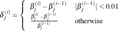
and
 is the estimate of the jth parameter at iteration i.
By default, XCONV=1E–4. You can also specify the ABSFCONV= and FCONV= criteria; if more than one criterion is specified, then optimizations are terminated as soon as one criterion is satisfied.