The GENMOD Procedure
-
Overview

-
Getting Started
-
SyntaxPROC GENMOD StatementASSESS StatementBAYES StatementBY StatementCLASS StatementCODE StatementCONTRAST StatementDEVIANCE StatementEFFECTPLOT StatementESTIMATE StatementEXACT StatementEXACTOPTIONS StatementFREQ StatementFWDLINK StatementINVLINK StatementLSMEANS StatementLSMESTIMATE StatementMODEL StatementOUTPUT StatementProgramming StatementsREPEATED StatementSLICE StatementSTORE StatementSTRATA StatementVARIANCE StatementWEIGHT StatementZEROMODEL Statement
-
DetailsGeneralized Linear Models TheorySpecification of EffectsParameterization Used in PROC GENMODType 1 AnalysisType 3 AnalysisConfidence Intervals for ParametersF StatisticsLagrange Multiplier StatisticsPredicted Values of the MeanResidualsMultinomial ModelsZero-Inflated ModelsTweedie Distribution For Generalized Linear ModelsGeneralized Estimating EquationsAssessment of Models Based on Aggregates of ResidualsCase Deletion Diagnostic StatisticsBayesian AnalysisExact Logistic and Exact Poisson RegressionMissing ValuesDisplayed Output for Classical AnalysisDisplayed Output for Bayesian AnalysisDisplayed Output for Exact AnalysisODS Table NamesODS Graphics
-
ExamplesLogistic RegressionNormal Regression, Log Link Gamma Distribution Applied to Life DataOrdinal Model for Multinomial DataGEE for Binary Data with Logit Link FunctionLog Odds Ratios and the ALR AlgorithmLog-Linear Model for Count DataModel Assessment of Multiple Regression Using Aggregates of ResidualsAssessment of a Marginal Model for Dependent DataBayesian Analysis of a Poisson Regression ModelExact Poisson RegressionTweedie Regression
- References
This is a brief introduction to the theory of generalized linear models.
In generalized linear models, the response is assumed to possess a probability distribution of the exponential form. That is, the probability density of the response Y for continuous response variables, or the probability function for discrete responses, can be expressed as
for some functions a, b, and c that determine the specific distribution. For fixed ![]() , this is a one-parameter exponential family of distributions. The functions a and c are such that
, this is a one-parameter exponential family of distributions. The functions a and c are such that ![]() and
and ![]() , where w is a known weight for each observation. A variable representing w in the input data set can be specified in the WEIGHT statement. If no WEIGHT statement is specified,
, where w is a known weight for each observation. A variable representing w in the input data set can be specified in the WEIGHT statement. If no WEIGHT statement is specified, ![]() for all observations.
for all observations.
Standard theory for this type of distribution gives expressions for the mean and variance of Y:
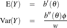
where the primes denote derivatives with respect to ![]() . If
. If ![]() represents the mean of Y, then the variance expressed as a function of the mean is
represents the mean of Y, then the variance expressed as a function of the mean is
where V is the variance function.
Probability distributions of the response Y in generalized linear models are usually parameterized in terms of the mean ![]() and dispersion parameter
and dispersion parameter ![]() instead of the natural parameter
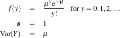
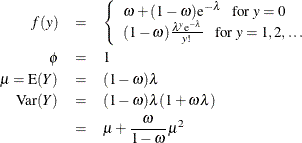
instead of the natural parameter ![]() . The probability distributions that are available in the GENMOD procedure are shown in the following list. The zero-inflated
Poisson and zero-inflated negative binomial distributions are not generalized linear models. However, the zero-inflated distributions
are included in PROC GENMOD since they are useful extensions of generalized linear models. See Long (1997) for a discussion of the zero-inflated Poisson and zero-inflated negative binomial distributions. The PROC GENMOD scale parameter
and the variance of Y are also shown.
. The probability distributions that are available in the GENMOD procedure are shown in the following list. The zero-inflated
Poisson and zero-inflated negative binomial distributions are not generalized linear models. However, the zero-inflated distributions
are included in PROC GENMOD since they are useful extensions of generalized linear models. See Long (1997) for a discussion of the zero-inflated Poisson and zero-inflated negative binomial distributions. The PROC GENMOD scale parameter
and the variance of Y are also shown.
![\begin{eqnarray*} f(y) & = & \frac{1}{\sqrt {2\pi } \sigma } \exp \left[ -\frac{1}{2} \left( \frac{y-\mu }{\sigma } \right)^2 \right]~ ~ ~ \mbox{for } -\infty < y < \infty \\ \phi & = & \sigma ^{2} \\ \mr {scale} & = & \sigma \\ \mr {Var}(Y) & = & \sigma ^{2} \\ \end{eqnarray*}](images/statug_genmod0176.png)
![\begin{eqnarray*} f(y) & = & \frac{1}{\sqrt {2\pi y^3} \sigma } \exp \left[ -\frac{1}{2y} \left( \frac{y-\mu }{\mu \sigma } \right)^2 \right]~ ~ ~ \mbox{for } 0 < y < \infty \\ \phi & = & \sigma ^2 \\ \mr {scale} & = & \sigma \\ \mr {Var}(Y) & = & \sigma ^2 \mu ^3 \\ \end{eqnarray*}](images/statug_genmod0177.png)
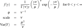
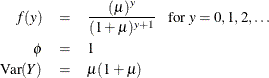
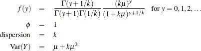

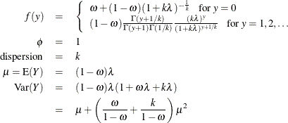
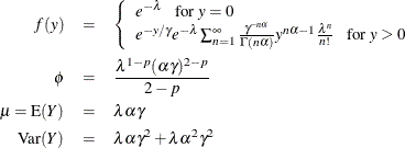
The negative binomial and the zero-inflated negative binomial distributions contain a parameter k, called the negative binomial dispersion parameter. This is not the same as the generalized linear model dispersion ![]() , but it is an additional distribution parameter that must be estimated or set to a fixed value.
, but it is an additional distribution parameter that must be estimated or set to a fixed value.
For the binomial distribution, the response is the binomial proportion ![]() .
The variance function is
.
The variance function is ![]() , and the binomial trials parameter n is regarded as a weight w.
, and the binomial trials parameter n is regarded as a weight w.
The density function for the Tweedie distribution when ![]() is expressed in terms of the parameters of the compound Poisson distribution. For more information about this representation,
see the section Tweedie Distribution For Generalized Linear Models. For
is expressed in terms of the parameters of the compound Poisson distribution. For more information about this representation,
see the section Tweedie Distribution For Generalized Linear Models. For ![]() , the Tweedie random variable has positive support and its density function
, the Tweedie random variable has positive support and its density function ![]() can be expressed in terms of stable distributions as defined in Hougaard (1986).
can be expressed in terms of stable distributions as defined in Hougaard (1986).
If a weight variable is present, ![]() is replaced with
is replaced with ![]() , where w is the weight variable.
, where w is the weight variable.
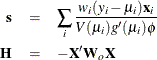
PROC GENMOD works with a scale parameter
that is related to the exponential family dispersion parameter ![]() instead of working with
instead of working with ![]() itself. The scale parameters are related to the dispersion parameter as shown previously with the probability distribution
definitions. Thus, the scale parameter output in the “Analysis of Parameter Estimates” table is related to the exponential family dispersion parameter. If you specify a constant scale parameter with the SCALE=
option in the MODEL statement, it is also related to the exponential family dispersion parameter in the same way.
itself. The scale parameters are related to the dispersion parameter as shown previously with the probability distribution
definitions. Thus, the scale parameter output in the “Analysis of Parameter Estimates” table is related to the exponential family dispersion parameter. If you specify a constant scale parameter with the SCALE=
option in the MODEL statement, it is also related to the exponential family dispersion parameter in the same way.
For distributions other than the zero-inflated Poisson or zero-inflated negative binomial, the mean ![]() of the response in the ith observation is related to a linear predictor through a monotonic differentiable link function g.
of the response in the ith observation is related to a linear predictor through a monotonic differentiable link function g.
Here, ![]() is a fixed known vector of explanatory variables, and
is a fixed known vector of explanatory variables, and ![]() is a vector of unknown parameters.
is a vector of unknown parameters.
There are two link functions and linear predictors associated with zero-inflated distributions: one for the zero inflation
probability ![]() , and another for the mean parameter
, and another for the mean parameter ![]() . See the section Zero-Inflated Models for more details about zero-inflated distributions.
. See the section Zero-Inflated Models for more details about zero-inflated distributions.
Log-likelihood functions for the distributions that are available in the procedure are parameterized in terms of the means
![]() and the dispersion parameter
and the dispersion parameter ![]() . Zero-inflated log likelihoods are parameterized in terms two parameters,
. Zero-inflated log likelihoods are parameterized in terms two parameters, ![]() and
and ![]() . The parameter
. The parameter ![]() is the zero-inflation probability, and
is the zero-inflation probability, and ![]() is a function of the distribution mean. The relationship between the mean of the zero-inflated Poisson and zero-inflated
negative binomial distributions and the parameter
is a function of the distribution mean. The relationship between the mean of the zero-inflated Poisson and zero-inflated
negative binomial distributions and the parameter ![]() is defined in the section Response Probability Distributions. The term
is defined in the section Response Probability Distributions. The term ![]() represents the response for the ith observation, and
represents the response for the ith observation, and ![]() represents the known dispersion weight. The log-likelihood functions are of the form
represents the known dispersion weight. The log-likelihood functions are of the form
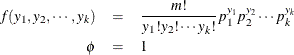
where the sum is over the observations. The forms of the individual contributions
are shown in the following list; the parameterizations are expressed in terms of the mean and dispersion parameters.
For the discrete distributions (binomial, multinomial, negative binomial, and Poisson), the functions computed as the sum
of the ![]() terms are not proper log-likelihood functions, since terms involving binomial coefficients or factorials of the observed
counts are dropped from the computation of the log likelihood, and a dispersion parameter
terms are not proper log-likelihood functions, since terms involving binomial coefficients or factorials of the observed
counts are dropped from the computation of the log likelihood, and a dispersion parameter ![]() is included in the computation. Deletion of factorial terms and inclusion of a dispersion parameter do not affect parameter
estimates or their estimated covariances for these distributions, and this is the function used in maximum likelihood estimation.
The value of
is included in the computation. Deletion of factorial terms and inclusion of a dispersion parameter do not affect parameter
estimates or their estimated covariances for these distributions, and this is the function used in maximum likelihood estimation.
The value of ![]() used in computing the reported log-likelihood function is either the final estimated value, or the fixed value, if the dispersion
parameter is fixed. Even though it is not a proper log-likelihood function in all cases, the function computed as the sum
of the
used in computing the reported log-likelihood function is either the final estimated value, or the fixed value, if the dispersion
parameter is fixed. Even though it is not a proper log-likelihood function in all cases, the function computed as the sum
of the ![]() terms is reported in the output as the log likelihood. The proper log-likelihood function is also computed as the sum of the
terms is reported in the output as the log likelihood. The proper log-likelihood function is also computed as the sum of the ![]() terms in the following list, and it is reported as the full log likelihood in the output.
terms in the following list, and it is reported as the full log likelihood in the output.
-
Normal:
![\[ \mathit{ll}_ i = l_ i = -\frac{1}{2} \left[ \frac{w_ i(y_ i-\mu _ i)^2}{\phi } + \log \left( \frac{\phi }{w_ i} \right) + \log (2 \pi ) \right] \]](images/statug_genmod0196.png)
-
Inverse Gaussian:
![\[ \mathit{ll}_ i = l_ i = -\frac{1}{2} \left[ \frac{w_ i(y_ i-\mu _ i)^2}{y_ i \mu ^2 \phi } + \log \left( \frac{\phi y_ i^3}{w_ i} \right) + \log (2 \pi ) \right] \]](images/statug_genmod0197.png)
-
Gamma:
![\[ \mathit{ll}_ i = l_ i = \frac{w_ i}{\phi } \log \left( \frac{w_ i y_ i}{\phi \mu _ i} \right) - \frac{w_ i y_ i}{\phi \mu _ i} - \log (y_ i) - \log \left( \Gamma \left( \frac{w_ i}{\phi } \right) \right) \]](images/statug_genmod0198.png)
-
Negative binomial:
![\[ l_ i = y_ i\log \left(\frac{k\mu }{w_ i} \right) - (y_ i+w_ i/k)\log \left(1+\frac{k\mu }{w_ i} \right) + \log \left(\frac{\Gamma (y_ i+w_ i/k)}{\Gamma (w_ i/k)}\right) \]](images/statug_genmod0199.png)
![\[ \mathit{ll}_ i = y_ i\log \left(\frac{k\mu }{w_ i} \right) - (y_ i+w_ i/k)\log \left(1+\frac{k\mu }{w_ i} \right) + \log \left(\frac{\Gamma (y_ i+w_ i/k)}{\Gamma (y_ i+1)\Gamma (w_ i/k)}\right) \]](images/statug_genmod0200.png)
-
Poisson:
![\[ l_ i = \frac{w_ i}{\phi }[y_ i \log (\mu _ i) - \mu _ i] \]](images/statug_genmod0201.png)
![\[ \mathit{ll}_ i = w_ i[y_ i \log (\mu _ i) - \mu _ i - \log (y_ i!) ] \]](images/statug_genmod0202.png)
-
Binomial:
![\[ l_ i = \frac{w_ i}{\phi }[r_ i \log (p_ i) + (n_ i-r_ i) \log (1-p_ i)] \]](images/statug_genmod0203.png)
![\[ \mathit{ll}_ i = w_ i[\log \left( \begin{array}{c} n_ i \\ r_ i \end{array} \right) + r_ i \log (p_ i) + (n_ i-r_ i) \log (1-p_ i)] \]](images/statug_genmod0204.png)
-
Multinomial (k categories):
![\[ l_ i = \frac{w_ i}{\phi }\sum _{j=1}^ k y_{ij}\log (\mu _{ij}) \]](images/statug_genmod0205.png)
![\[ \mathit{ll}_ i = w_ i[\log (m_ i!)+\sum _{j=1}^ k (y_{ij}\log (\mu _{ij})-\log (y_{ij}!))] \]](images/statug_genmod0206.png)
-
Zero-inflated Poisson:
![\[ l_ i = \mathit{ll}_ i = \left\{ \begin{array}{ll} w_ i\log [\omega _ i + (1-\omega _ i)\exp (-\lambda _ i)] & y_ i=0 \\ w_ i[\log (1-\omega _ i)+y_ i \log (\lambda _ i) - \lambda _ i-\log (y_ i!)] & y_ i>0 \\ \end{array} \right. \]](images/statug_genmod0207.png)
-
Zero-inflated negative binomial:
![\[ l_ i = \mathit{ll}_ i = \left\{ \begin{array}{ll} \log [\omega _ i + (1-\omega _ i)(1+\frac{k}{w_ i}\lambda )^{-\frac{1}{k}}] & y_ i=0 \\ \log (1-\omega _ i)+ y_ i\log \left(\frac{k\lambda }{w_ i} \right) & \\ -(y_ i+\frac{w_ i}{k})\log \left(1+\frac{k\lambda }{w_ i} \right) & \\ +\log \left(\frac{\Gamma (y_ i+\frac{w_ i}{k})}{\Gamma (y_ i+1)\Gamma (\frac{w_ i}{k})}\right) & y_ i>0 \\ \end{array} \right. \]](images/statug_genmod0208.png)
-
Tweedie:
![\[ l_ i = \mathit{ll}_ i = \log \left( f(y_ i,\mu _ i ,\phi /\omega _ i, p) \right) \]](images/statug_genmod0209.png)
The GENMOD procedure uses a ridge-stabilized Newton-Raphson algorithm
to maximize the log-likelihood function ![]() with respect to the regression parameters.
By default, the procedure also produces maximum likelihood estimates of the scale parameter as defined in the section Response Probability Distributions for the normal, inverse Gaussian, negative binomial, and gamma distributions.
with respect to the regression parameters.
By default, the procedure also produces maximum likelihood estimates of the scale parameter as defined in the section Response Probability Distributions for the normal, inverse Gaussian, negative binomial, and gamma distributions.
On the rth iteration, the algorithm updates the parameter vector ![]() with
with
where ![]() is the Hessian
(second derivative) matrix, and
is the Hessian
(second derivative) matrix, and ![]() is the gradient
(first derivative) vector of the log-likelihood function, both evaluated at the current value of the parameter vector. That
is,
is the gradient
(first derivative) vector of the log-likelihood function, both evaluated at the current value of the parameter vector. That
is,
and
In some cases, the scale parameter is estimated by maximum likelihood. In these cases, elements corresponding to the scale
parameter are computed and included in ![]() and
and ![]() .
.
If ![]() is the linear predictor for observation i and g is the link function, then
is the linear predictor for observation i and g is the link function, then ![]() , so that
, so that ![]() is an estimate of the mean of the ith observation, obtained from an estimate of the parameter vector
is an estimate of the mean of the ith observation, obtained from an estimate of the parameter vector ![]() .
.
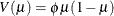
The gradient vector and Hessian matrix for the regression parameters are given by
where ![]() is the design matrix,
is the design matrix, ![]() is the transpose of the ith row of X, and V is the variance function. The matrix
is the transpose of the ith row of X, and V is the variance function. The matrix ![]() is diagonal with its ith diagonal element
is diagonal with its ith diagonal element
where
The primes denote derivatives of g and V with respect to ![]() . The negative of
. The negative of ![]() is called the observed information matrix.
The expected value of
is called the observed information matrix.
The expected value of ![]() is a diagonal matrix
is a diagonal matrix ![]() with diagonal values
with diagonal values ![]() . If you replace
. If you replace ![]() with
with ![]() , then the negative of
, then the negative of ![]() is called the expected information matrix.
is called the expected information matrix.
![]() is the weight matrix for the Fisher scoring
method of fitting. Either
is the weight matrix for the Fisher scoring
method of fitting. Either ![]() or
or ![]() can be used in the update equation. The GENMOD procedure uses Fisher scoring for iterations up to the number specified by
the SCORING option in the MODEL statement, and it uses the observed information matrix on additional iterations.
can be used in the update equation. The GENMOD procedure uses Fisher scoring for iterations up to the number specified by
the SCORING option in the MODEL statement, and it uses the observed information matrix on additional iterations.
The estimated covariance matrix of the parameter estimator is given by
where ![]() is the Hessian matrix evaluated using the parameter estimates on the last iteration. Note that the dispersion parameter,
whether estimated or specified, is incorporated into
is the Hessian matrix evaluated using the parameter estimates on the last iteration. Note that the dispersion parameter,
whether estimated or specified, is incorporated into ![]() . Rows and columns corresponding to aliased parameters are not included in
. Rows and columns corresponding to aliased parameters are not included in ![]() .
.
The correlation matrix
is the normalized covariance matrix. That is, if ![]() is an element of
is an element of ![]() , then the corresponding element of the correlation matrix is
, then the corresponding element of the correlation matrix is ![]() , where
, where ![]() .
.
Two statistics that are helpful in assessing the goodness of fit
of a given generalized linear model are the scaled deviance
and Pearson’s chi-square statistic.
For a fixed value of the dispersion parameter ![]() , the scaled deviance is defined to be twice the difference between the maximum achievable log likelihood and the log likelihood
at the maximum likelihood estimates of the regression parameters.
, the scaled deviance is defined to be twice the difference between the maximum achievable log likelihood and the log likelihood
at the maximum likelihood estimates of the regression parameters.
Note that these statistics are not valid for GEE models.
If ![]() is the log-likelihood function expressed as a function of the predicted mean values
is the log-likelihood function expressed as a function of the predicted mean values ![]() and the vector
and the vector ![]() of response values, then the scaled deviance
is defined by
of response values, then the scaled deviance
is defined by
For specific distributions, this can be expressed as
where D is the deviance. The following table displays the deviance for each of the probability distributions available in PROC GENMOD. The deviance cannot be directly calculated for zero-inflated models. Twice the negative of the log likelihood is reported instead of the proper deviance for the zero-inflated Poisson and zero-inflated negative binomial.
|
Distribution |
Deviance |
|---|---|
|
Normal |
|
|
Poisson |
|
|
Binomial |
|
|
Gamma |
|
|
Inverse Gaussian |
|
|
Multinomial |
|
|
Negative binomial |
|
|
Zero-inflated Poisson |
|
|
Zero-inflated negative binomial |
|
![$ -2\sum _ i\left\{ \begin{array}{ll} w_ i\log [\omega _ i + (1-\omega _ i)\exp (-\mu _ i)] & y_ i=0 \\ w_ i[\log (1-\omega _ i)+y_ i \log (\mu _ i) - & \\ \mu _ i-\log (y_ i!)] & y_ i>0 \\ \end{array} \right. $](images/statug_genmod0240.png)
![$ -2\sum _ i\left\{ \begin{array}{lll} \log [\omega _ i + (1-\omega _ i)(1+\frac{k}{w_ i}\lambda )] & y_ i=0 \\ \log (1-\omega _ i)+ y_ i\log \left(\frac{k\lambda }{w_ i} \right) - & \\ (y_ i+\frac{w_ i}{k})\log \left(1+\frac{k\lambda }{w_ i} \right) + & \\ \log \left(\frac{\Gamma (y_ i+\frac{w_ i}{k})}{\Gamma (y_ i+1)\Gamma (\frac{w_ i}{k})}\right) & y_ i>0 \\ \end{array} \right. $](images/statug_genmod0241.png)
In the binomial case, ![]() , where
, where ![]() is a binomial count and
is a binomial count and ![]() is the binomial number of trials parameter.
is the binomial number of trials parameter.
In the multinomial case, ![]() refers to the observed number of occurrences of the jth category for the ith subpopulation defined by the AGGREGATE= variable,
refers to the observed number of occurrences of the jth category for the ith subpopulation defined by the AGGREGATE= variable, ![]() is the total number in the ith subpopulation, and
is the total number in the ith subpopulation, and ![]() is the category probability.
is the category probability.
Pearson’s chi-square statistic is defined as
and the scaled Pearson’s chi-square is ![]() .
.
The scaled version of both of these statistics, under certain regularity conditions, has a limiting chi-square distribution, with degrees of freedom equal to the number of observations minus the number of parameters estimated. The scaled version can be used as an approximate guide to the goodness of fit of a given model. Use caution before applying these statistics to ensure that all the conditions for the asymptotic distributions hold. McCullagh and Nelder (1989) advise that differences in deviances for nested models can be better approximated by chi-square distributions than the deviances can themselves.
In cases where the dispersion parameter is not known, an estimate can be used to obtain an approximation to the scaled deviance
and Pearson’s chi-square statistic. One strategy is to fit a model that contains a sufficient number of parameters so that
all systematic variation is removed, estimate ![]() from this model, and then use this estimate in computing the scaled deviance of submodels. The deviance or Pearson’s chi-square
divided by its degrees of freedom is sometimes used as an estimate
of the dispersion parameter
from this model, and then use this estimate in computing the scaled deviance of submodels. The deviance or Pearson’s chi-square
divided by its degrees of freedom is sometimes used as an estimate
of the dispersion parameter ![]() . For example, since the limiting chi-square distribution of the scaled deviance
. For example, since the limiting chi-square distribution of the scaled deviance ![]() has
has ![]() degrees of freedom, where n is the number of observations and p is the number of parameters, equating
degrees of freedom, where n is the number of observations and p is the number of parameters, equating ![]() to its mean and solving for
to its mean and solving for ![]() yields
yields ![]() . Similarly, an estimate of
. Similarly, an estimate of ![]() based on Pearson’s chi-square
based on Pearson’s chi-square ![]() is
is ![]() . Alternatively, a maximum likelihood estimate of
. Alternatively, a maximum likelihood estimate of ![]() can be computed by the procedure, if desired. See the discussion in the section Type 1 Analysis for more about the estimation of the dispersion parameter.
can be computed by the procedure, if desired. See the discussion in the section Type 1 Analysis for more about the estimation of the dispersion parameter.
The Akaike information criterion (AIC) is a measure of goodness of model fit that balances model fit against model simplicity. AIC has the form
where p is the number of parameters estimated in the model, and LL is the log likelihood evaluated at the value of the estimated parameters. An alternative form is the corrected AIC given by
where n is the total number of observations used.
The Bayesian information criterion (BIC) is a similar measure. BIC is defined by
See Akaike (1981, 1979) for details of AIC and BIC. See Simonoff (2003) for a discussion of using AIC, AICC, and BIC with generalized linear models. These criteria are useful in selecting among regression models, with smaller values representing better model fit. PROC GENMOD uses the full log likelihoods defined in the section Log-Likelihood Functions, with all terms included, for computing all of the criteria.
There are several options available in PROC GENMOD for handling the exponential distribution dispersion parameter. The NOSCALE and SCALE options in the MODEL statement affect the way in which the dispersion parameter is treated. If you specify the SCALE=DEVIANCE option, the dispersion parameter is estimated by the deviance divided by its degrees of freedom. If you specify the SCALE=PEARSON option, the dispersion parameter is estimated by Pearson’s chi-square statistic divided by its degrees of freedom.
Otherwise, values of the SCALE and NOSCALE options and the resultant actions are displayed in the following table.
|
NOSCALE |
SCALE=value |
Action |
|---|---|---|
|
Present |
Present |
Scale fixed at value |
|
Present |
Not present |
Scale fixed at 1 |
|
Not present |
Not present |
Scale estimated by ML |
|
Not present |
Present |
Scale estimated by ML, |
|
starting point at value |
||
|
Present (negative binomial) |
Not present |
k fixed at 0 |
The meaning of the scale parameter displayed in the “Analysis Of Parameter Estimates” table is different for the gamma distribution than for the other distributions. The relation of the scale parameter as used
by PROC GENMOD to the exponential family dispersion parameter ![]() is displayed in the following table. For the binomial and Poisson distributions,
is displayed in the following table. For the binomial and Poisson distributions, ![]() is the overdispersion parameter, as defined in the “Overdispersion” section, which follows.
is the overdispersion parameter, as defined in the “Overdispersion” section, which follows.
|
Distribution |
Scale |
|---|---|
|
Normal |
|
|
Inverse Gaussian |
|
|
Gamma |
|
|
Binomial |
|
|
Poisson |
|
In the case of the negative binomial distribution, PROC GENMOD reports the “dispersion” parameter estimated by maximum likelihood. This is the negative binomial parameter k defined in the section Response Probability Distributions.
Overdispersion
is a phenomenon that sometimes occurs in data that are modeled with the binomial or Poisson distributions. If the estimate
of dispersion after fitting, as measured by the deviance or Pearson’s chi-square, divided by the degrees of freedom, is not
near 1, then the data might be overdispersed if the dispersion estimate is greater than 1 or underdispersed if the dispersion estimate is less than 1. A simple way to model this situation is to allow the variance functions of these
distributions to have a multiplicative overdispersion factor ![]() :
:
-
Binomial:
-
Poisson:

An alternative method to allow for overdispersion in the Poisson distribution is to fit a negative binomial distribution,
where ![]() , instead of the Poisson. The parameter k can be estimated by maximum likelihood, thus allowing for overdispersion of a specific form. This is different from the multiplicative
overdispersion factor
, instead of the Poisson. The parameter k can be estimated by maximum likelihood, thus allowing for overdispersion of a specific form. This is different from the multiplicative
overdispersion factor ![]() , which can accommodate many forms of overdispersion.
, which can accommodate many forms of overdispersion.
The models are fit in the usual way, and the parameter estimates are not affected by the value of ![]() . The covariance matrix, however, is multiplied by
. The covariance matrix, however, is multiplied by ![]() , and the scaled deviance and log likelihoods used in likelihood ratio tests are divided by
, and the scaled deviance and log likelihoods used in likelihood ratio tests are divided by ![]() . The profile likelihood function used in computing confidence intervals is also divided by
. The profile likelihood function used in computing confidence intervals is also divided by ![]() . If you specify a WEIGHT statement,
. If you specify a WEIGHT statement, ![]() is divided by the value of the WEIGHT variable for each observation. This has the effect of multiplying the contributions
of the log-likelihood function, the gradient, and the Hessian by the value of the WEIGHT variable for each observation.
is divided by the value of the WEIGHT variable for each observation. This has the effect of multiplying the contributions
of the log-likelihood function, the gradient, and the Hessian by the value of the WEIGHT variable for each observation.
The SCALE= option in the MODEL statement enables you to specify a value of ![]() for the binomial and Poisson distributions. If you specify the SCALE=DEVIANCE option in the MODEL statement, the procedure
uses the deviance divided by degrees of freedom as an estimate of
for the binomial and Poisson distributions. If you specify the SCALE=DEVIANCE option in the MODEL statement, the procedure
uses the deviance divided by degrees of freedom as an estimate of ![]() , and all statistics are adjusted appropriately. You can use Pearson’s chi-square instead of the deviance by specifying the
SCALE=PEARSON option.
, and all statistics are adjusted appropriately. You can use Pearson’s chi-square instead of the deviance by specifying the
SCALE=PEARSON option.
The function obtained by dividing a log-likelihood function for the binomial or Poisson distribution by a dispersion parameter is not a legitimate log-likelihood function. It is an example of a quasi-likelihood function. Most of the asymptotic theory for log likelihoods also applies to quasi-likelihoods, which justifies computing standard errors and likelihood ratio statistics by using quasi-likelihoods instead of proper log likelihoods. For details on quasi-likelihood functions, see McCullagh and Nelder (1989, Chapter 9), McCullagh (1983); Hardin and Hilbe (2003).
Although the estimate of the dispersion parameter is often used to indicate overdispersion or underdispersion, this estimate might also indicate other problems such as an incorrectly specified model or outliers in the data. You should carefully assess whether this type of model is appropriate for your data.