The GENMOD Procedure
-
Overview

-
Getting Started
-
SyntaxPROC GENMOD StatementASSESS StatementBAYES StatementBY StatementCLASS StatementCODE StatementCONTRAST StatementDEVIANCE StatementEFFECTPLOT StatementESTIMATE StatementEXACT StatementEXACTOPTIONS StatementFREQ StatementFWDLINK StatementINVLINK StatementLSMEANS StatementLSMESTIMATE StatementMODEL StatementOUTPUT StatementProgramming StatementsREPEATED StatementSLICE StatementSTORE StatementSTRATA StatementVARIANCE StatementWEIGHT StatementZEROMODEL Statement
-
DetailsGeneralized Linear Models TheorySpecification of EffectsParameterization Used in PROC GENMODType 1 AnalysisType 3 AnalysisConfidence Intervals for ParametersF StatisticsLagrange Multiplier StatisticsPredicted Values of the MeanResidualsMultinomial ModelsZero-Inflated ModelsTweedie Distribution For Generalized Linear ModelsGeneralized Estimating EquationsAssessment of Models Based on Aggregates of ResidualsCase Deletion Diagnostic StatisticsBayesian AnalysisExact Logistic and Exact Poisson RegressionMissing ValuesDisplayed Output for Classical AnalysisDisplayed Output for Bayesian AnalysisDisplayed Output for Exact AnalysisODS Table NamesODS Graphics
-
ExamplesLogistic RegressionNormal Regression, Log Link Gamma Distribution Applied to Life DataOrdinal Model for Multinomial DataGEE for Binary Data with Logit Link FunctionLog Odds Ratios and the ALR AlgorithmLog-Linear Model for Count DataModel Assessment of Multiple Regression Using Aggregates of ResidualsAssessment of a Marginal Model for Dependent DataBayesian Analysis of a Poisson Regression ModelExact Poisson RegressionTweedie Regression
- References
The Tweedie (1984) distribution has nonnegative support and can have a discrete mass at zero, making it useful to model responses that are
a mixture of zeros and positive values. The Tweedie distribution belongs to the exponential family, so it conveniently fits
in the generalized linear models framework. According to such parameterization, the mean and variance for the Tweedie random
variable are ![]() and
and ![]() , respectively, where
, respectively, where ![]() is the dispersion parameter and
is the dispersion parameter and ![]() is an extra parameter that controls the variance of the distribution.
is an extra parameter that controls the variance of the distribution.
The Tweedie family of distributions includes several important distributions for generalized linear models. When ![]() , the Tweedie distribution degenerates to the normal distribution; when
, the Tweedie distribution degenerates to the normal distribution; when ![]() , it becomes a Poisson distribution; when
, it becomes a Poisson distribution; when ![]() , it becomes a gamma distribution; when
, it becomes a gamma distribution; when ![]() , it is an inverse Gaussian distribution.
, it is an inverse Gaussian distribution.
Except for these special cases, the probability density function for the Tweedie distribution does not have a closed form
and can at best be expressed in terms of series. Numerical approximations are needed to evaluate the density function. Dunn
and Smyth (2005) propose using a finite series and provide a formula to determine its lower and upper indices in order to achieve a desired
accuracy. Alternatively, you can apply the Fourier transformation on the characteristic function (Dunn and Smyth, 2008). These approximations tend to be expensive when a high level of accuracy is demanded or the data volume becomes large. PROC
GENMOD uses the series method unless it becomes complicated to do so. In this case, the method that is based on the Fourier
transformation is used. The accuracy of approximation is controlled by the EPSILON= option, whose default value is ![]() .
.
The Tweedie distribution is not defined when ![]() is between 0 and 1. In practice, the most interesting range is from 1 to 2 in which the Tweedie distribution gradually loses
its mass at 0 as it shifts from a Poisson distribution to a gamma distribution. In this case, the Tweedie random variable
is between 0 and 1. In practice, the most interesting range is from 1 to 2 in which the Tweedie distribution gradually loses
its mass at 0 as it shifts from a Poisson distribution to a gamma distribution. In this case, the Tweedie random variable
![]() can be generated from a compound Poisson distribution (Smyth, 1996) as
can be generated from a compound Poisson distribution (Smyth, 1996) as
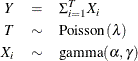
where ![]() if
if ![]() ,
, ![]() and
and ![]() are statistically independent, and
are statistically independent, and ![]() denotes a gamma random variable that has mean
denotes a gamma random variable that has mean ![]() and variance
and variance ![]() . These parameters are determined by the Tweedie parameters as follows:
. These parameters are determined by the Tweedie parameters as follows:
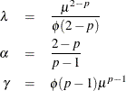
Inversely, given the Tweedie distributional parameters, the parameters of the compound Poisson distribution are determined as follows:
In terms of generalized linear models parameterizations, the canonical parameter ![]() for the Tweedie density can be expressed as
for the Tweedie density can be expressed as
and the function ![]() is
is
Because of the intractability of differentiating the gradient functions with respect to the variance parameters, PROC GENMOD
uses a quasi-Newton approach to maximize the likelihood function, where the Hessian matrix is approximated by taking finite
differences of the gradient functions. Convergence is determined by a union of two criteria: the relative gradient convergence
criterion is set to ![]() , and the relative function convergence criterion is set to
, and the relative function convergence criterion is set to ![]() . Convergence is declared when at least one of the criteria is attained during the quasi-Newton iteration.
. Convergence is declared when at least one of the criteria is attained during the quasi-Newton iteration.
Before PROC GENMOD maximizes the approximate likelihood, it first maximizes the following extended log quasi-likelihood which is constructed according to the definition of McCullagh and Nelder (1989, Chapter 9) as
where the contribution from an observation is
and ![]() is the weight for the observation from the WEIGHT statement.
is the weight for the observation from the WEIGHT statement.
The range of parameter ![]() for the quasi-likelihood is from 1 to 2. For a specified P= value outside this range, PROC GENMOD skips optimization of the
quasi-likelihood. To maintain numerical stability, PROC GENMOD imposes a lower bound of 1.1 and a upper bound of 1.99 for
computation with the quasi-likelihood. The estimates that are obtained from optimizing the quasi-likelihood are usually near
the full-likelihood solution so that fewer iterations are needed for maximizing the more expensive full likelihood.
for the quasi-likelihood is from 1 to 2. For a specified P= value outside this range, PROC GENMOD skips optimization of the
quasi-likelihood. To maintain numerical stability, PROC GENMOD imposes a lower bound of 1.1 and a upper bound of 1.99 for
computation with the quasi-likelihood. The estimates that are obtained from optimizing the quasi-likelihood are usually near
the full-likelihood solution so that fewer iterations are needed for maximizing the more expensive full likelihood.