The PHREG Procedure
- Overview
-
Getting Started

-
Syntax
PROC PHREG Statement ASSESS Statement BASELINE Statement BAYES Statement BY Statement CLASS Statement CONTRAST Statement EFFECT Statement ESTIMATE Statement FREQ Statement HAZARDRATIO Statement ID Statement LSMEANS Statement LSMESTIMATE Statement MODEL Statement OUTPUT Statement Programming Statements RANDOM Statement STRATA Statement SLICE Statement STORE Statement TEST Statement WEIGHT Statement
-
Details
Failure Time Distribution Time and CLASS Variables Usage Partial Likelihood Function for the Cox Model Counting Process Style of Input Left-Truncation of Failure Times The Multiplicative Hazards Model The Frailty Model Hazard Ratios Specifics for Classical Analysis Specifics for Bayesian Analysis Computational Resources Input and Output Data Sets Displayed Output ODS Table Names ODS Graphics
-
Examples
Stepwise Regression Best Subset Selection Modeling with Categorical Predictors Firth’s Correction for Monotone Likelihood Conditional Logistic Regression for m:n Matching Model Using Time-Dependent Explanatory Variables Time-Dependent Repeated Measurements of a Covariate Survivor Function Estimates for Specific Covariate Values Analysis of Residuals Analysis of Recurrent Events Data Analysis of Clustered Data Model Assessment Using Cumulative Sums of Martingale Residuals Bayesian Analysis of the Cox Model Bayesian Analysis of Piecewise Exponential Model
- References
| The Frailty Model |
You can use the frailty model to model correlations between failures of the same cluster by using a random component for the hazard function. The hazard rate for the  th individual in the
  th cluster is
 |
where  is an arbitrary baseline hazard rate,
  is the vector of (fixed-effect) covariates,
  is the vector of regression coefficients, and
  is the random effect for cluster . The random components
  are assumed to be independent and identically distributed as a normal random variable with mean 0 and an unknown variance
  .
.
In terms of the frailties  , given by
  , the frailty model can be written as
 |
Each frailty has a lognormal distribution with median 1. This gives the interpretation that individuals in cluster with  tend to fail at a faster (slower) rate than that under an independence model.
The RANDOM statement in PROC PHREG enables you to fit a shared fraity model. However, the ASSESS, BASELINE, and OUTPUT statements, if specified, are ignored. Also ignored are the COVS options in the PROC PHREG statement and the following options in the MODEL statement: BEST=, DETAILS, HIERARCHY=, INCLUDE=, NOFIT, PLCONV=, SELECTION=, SEQUENTIAL, SLENTRY=, SLSTAY=, TYPE1, and TYPE3(ALL, LR, SCORE). Profile likelihood confidence intervals for the hazard ratios are not available for the frailty model analysis.
The Penalized Partial Likelihood Approach for Fitting Frailty Models
Let  be the vector of random components for the
  clusters. With each having a zero-mean normal distribution and a common variance , the joint log likelihood is
 |
Define the penalized partial log likelihood as
 |
where  is the log of any of the partial likelihood in the sections Partial Likelihood Function for the Cox Model and The Multiplicative Hazards Model.
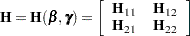
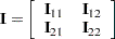
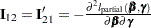
For a given , let  be the negative Hessian of the penalized partial log likelihood
  ; that is,
 |
where 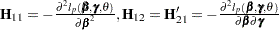 , and
, and 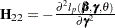 .
.
The marginal log likelihood of this shared frailty model is
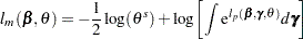 |
Using a Laplace approximation to the integral as in Breslow and Clayton (1993), an approximate marginal log likelihood (Ripatti and Palmgren; 2000; Therneau and Grambsch; 2000) is given by
 |
The maximization of this approximate likelihood is a doubly iterative process that alternates between the following two steps:
For a provisional value of
, PROC PHREG computes the best linear unbiased predictors (BLUP) of and  by maximizing the penalized partial log likelihood . This contitutes the inner loop.
 For
and fixed at the BLUP values, PROC PHREG estimates by maximizing the approximate marginal likelihood  . This constitutes the outer loop.
The outer loop is iterated until the difference between two successive estimates of is small.
The ML estimate of is
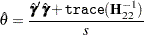 |
The variance for  is
is
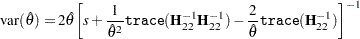 |
The REML estimation of is obtained by replacing  by
by  .
.
The inverse of the final matrix is used as the variance estimate of  .
.
The final BLUP estimates of the random components can be displayed using the SOLUTION option in the RANDOM statement. Also displayed are estimates of the lognormal frailties, which are the exponentiated estimates of the BLUP estimates.
Wald-Type Tests for Penalized Models
Let  be the negative Hessian of the partial log likelihood
  :
:
 |
where 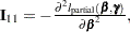
 , and
, and 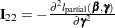 . Write
  . The Wald-type chi-square statistic for testing
  is
is
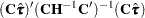 |
Let  . Gray (1992) recommends the following generalized degrees of freedom for the Wald test:
 |
See Therneau and Grambsch (2000, Section 5.8) for a discussion of this Wald-type test.
PROC PHREG uses the label "Adjusted DF" to represent this generalized degrees of freedom in the output.