The NLIN Procedure
- Overview
-
Getting Started

-
Syntax
-
Details
Automatic Derivatives Measures of Nonlinearity and Diagnostics Missing Values Special Variables Troubleshooting Computational Methods Output Data Sets Confidence Intervals Covariance Matrix of Parameter Estimates Convergence Measures Displayed Output Incompatibilities with SAS 6.11 and Earlier Versions of PROC NLIN ODS Table Names ODS Graphics
-
Examples
- References
Example 62.4 Affecting Curvature through Parameterization
The work of Ratkowksy (1983, 1990) has brought into focus the importance of close-to-linear behavior of parameters in nonlinear regression models. The curvature in a nonlinear model consists of two components: the intrinsic curvature and the parameter-effects curvature. See the section Relative Curvature Measures of Nonlinearity for details. Intrinsic curvature expresses the degree to which the nonlinear model bends as values of the parameters change. This is not the same as the curviness of the model as a function of the covariates (the  variables). Intrinsic curvature is a function of the type of model you are fitting and the data. This curvature component cannot be affected by reparameterization of the model. According to Ratkowsky (1983), the intrinsic curvature component is typically smaller than the parameter-effects curvature, which can be affected by altering the parameterization of the model.
In models with low curvature, the nonlinear least squares parameter estimators behave similarly to least squares estimators in linear regression models, which have a number of desirable properties. If the model is correct, they are best linear unbiased estimators and are normally distributed if the model errors are normal (otherwise they are asymptotically normal). As you lower the curvature of a nonlinear model, you can expect that the parameter estimators approach the behavior of the linear regression model estimators: they behave "close to linear."
This example uses a simple data set and a commonly applied model for dose-response relationships to examine how the parameter-effects curvature can be reduced. The statistics by which an estimator’s behavior is judged are Box’s bias (Box 1971) and Hougaard’s measure of skewness (Hougaard 1982, 1985).
The log-logistic model
 |
is a popular model to express the response  as a function of dose . The response is bounded between the asymptotes
  and
and  . The term in the denominator governs the transition between the asymptotes and depends on two parameters,
  and
and  . The log-logistic model can be viewed as a member of a broader class of dose-response functions, those relying on switch-on or switch-off mechanisms (see, for example, Schabenberger and Pierce 2002, sec. 5.8.6). A switch function is usually a monotonic function
  that takes values between 0 and 1. A switch-on function increases in ; a switch-off function decreases in . In the log-logistic case, the function
 |
is a switch-off function for  and a switch-on function for
  . You can write general dose-response functions with asymptotes simply as
 |
The following DATA step creates a small data set from a dose-response experiment with response y:
data logistic;
   input dose y;
   logdose = log(dose);
   datalines;
0.009  106.56
0.035   94.12
0.07    89.76
0.15    60.21
0.20    39.95
0.28    21.88
0.50     7.46
;
A graph of these data is produced with the following statements:
proc sgplot data=logistic;
   scatter y=y x=dose;
   xaxis type=log logstyle=linear;
run;
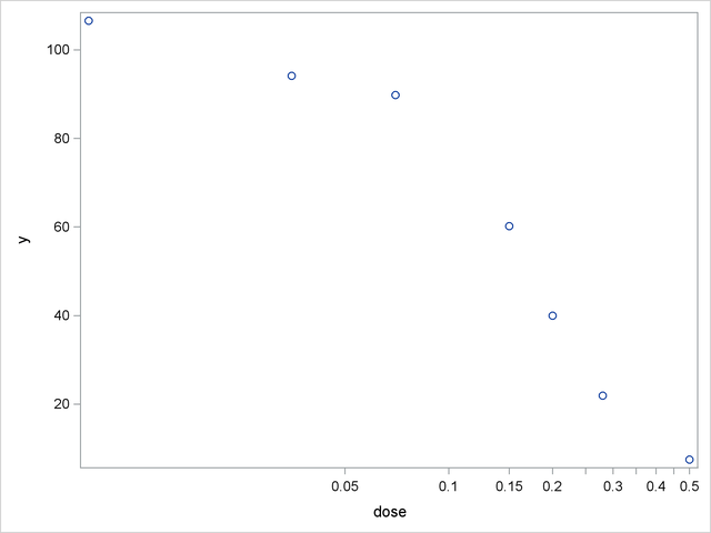
When dose is expressed on the log scale, the sigmoidal shape of the dose-response relationship is clearly visible (Output 62.4.1). The log-logistic switching model in the preceding parameterization is fit with the following statements in the NLIN procedure:
proc nlin data=logistic bias hougaard nlinmeasures;
   parameters alpha=100 beta=3 gamma=300;
   delta = 0;
   Switch = 1/(1+gamma*exp(beta*log(dose)));
   model y = delta + (alpha - delta)*Switch;
run;
The lower asymptote is assumed to be 0 in this case. Since is not listed in the PARAMETERS statement and is assigned a value in the program, it is assumed to be constant. Note that the term Switch is the switch-off function in the log-logistic model. The BIAS and HOUGAARD options in the PROC NLIN statement request that Box’s bias, percentage bias, and Hougaard’s skewness measure be added to the table of parameter estimates, and the NLINMEASURES option requests that the global nonlinearity measures be produced.
The NLIN procedure converges after  iterations and achieves a residual mean squared error of
  (Output 62.4.2). This value is not that important by itself, but it is worth noting since this model fit is compared to the fit with other parameterizations later on.
| Iterative Phase | ||||
|---|---|---|---|---|
| Iter | alpha | beta | gamma | Sum of Squares |
| 0 | 100.0 | 3.0000 | 300.0 | 386.4 |
| 1 | 100.4 | 2.8011 | 162.8 | 129.1 |
| 2 | 100.8 | 2.6184 | 101.4 | 69.2710 |
| 3 | 101.3 | 2.4266 | 69.7579 | 68.2167 |
| 4 | 101.7 | 2.3790 | 69.0358 | 60.8223 |
| 5 | 101.8 | 2.3621 | 67.3709 | 60.7516 |
| 6 | 101.8 | 2.3582 | 67.0044 | 60.7477 |
| 7 | 101.8 | 2.3573 | 66.9150 | 60.7475 |
| 8 | 101.8 | 2.3571 | 66.8948 | 60.7475 |
| 9 | 101.8 | 2.3570 | 66.8902 | 60.7475 |
| 10 | 101.8 | 2.3570 | 66.8892 | 60.7475 |
| NOTE: Convergence criterion met. |
| Note: | An intercept was not specified for this model. |
| Source | DF | Sum of Squares | Mean Square | F Value | Approx Pr > F |
|---|---|---|---|---|---|
| Model | 3 | 33965.4 | 11321.8 | 745.50 | <.0001 |
| Error | 4 | 60.7475 | 15.1869 | ||
| Uncorrected Total | 7 | 34026.1 |
The table of parameter estimates displays the estimates of the three model parameters, their approximate standard errors, 95% confidence limits, Hougaard’s skewness measure, Box’s bias, and percentage bias (Output 62.4.3). Parameters for which the skewness measure is less than 0.1 in absolute value and with percentage bias less than  exhibit very close-to-linear behavior, and skewness values less than
  in absolute value indicate reasonably close-to-linear behavior (Ratkowsky 1990). According to these rules, the estimators
  and
and  suffer from substantial curvature. The estimator is especially "far-from-linear." Inferences that involve and rely on the reported standard errors or confidence limits (or both) for this parameter might be questionable.
| Parameter | Estimate | Approx Std Error |
Approximate 95% Confidence Limits |
Skewness | Bias | Percent Bias |
|
|---|---|---|---|---|---|---|---|
| alpha | 101.8 | 3.0034 | 93.4751 | 110.2 | 0.1415 | 0.1512 | 0.15 |
| beta | 2.3570 | 0.2928 | 1.5440 | 3.1699 | 0.4987 | 0.0303 | 1.29 |
| gamma | 66.8892 | 31.6146 | -20.8870 | 154.7 | 1.9200 | 10.9230 | 16.3 |
The related global nonlinearity measures output table (Output 62.4.4) shows that both the maximum and RMS parameter-effects curvature are substantially larger than the critical curvature value recommended by Bates and Watts (1980). In contrast, the intrinsic curvatures of the model are less than the critical value. This implies that most of the nonlinearity can be removed by reparameterization.
| Global Nonlinearity Measures | |
|---|---|
| Max Intrinsic Curvature | 0.2397 |
| RMS Intrinsic Curvature | 0.1154 |
| Max Parameter-Effects Curvature | 4.0842 |
| RMS Parameter-Effects Curvature | 1.8198 |
| Curvature Critical Value | 0.3895 |
| Raw Residual Variance | 15.187 |
| Projected Residual Variance | 5.922 |
One method of reducing the parameter-effects curvature, and thereby reduce the bias and skewness of the parameter estimators, is to replace a parameter with its expected-value parameterization. Schabenberger et al. (1999) and Schabenberger and Pierce (2002, sec. 5.7.2) refer to this method as reparameterization through defining relationships. A defining relationship is obtained by equating the mean response at a chosen value of (say,  ) to the model:
 |
This equation is then solved for a parameter that is subsequently replaced in the original equation. This method is particularly useful if has an interesting interpretation. For example, let  denote the value that reduces the response by
  %,
%,
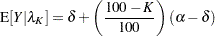 |
Because exhibits large bias and skewness, it is the target in the first round of reparameterization. Setting the expression for the conditional mean at equal to the mean function when  yields the following expression:
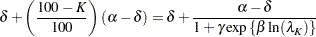 |
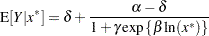
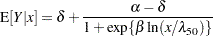
This expression is solved for , and the result is substituted back into the model equation. This leads to a log-logistic model in which is replaced by the parameter , the dose at which the response was reduced by %. The new model equation is
 |
A particularly interesting choice is  , since
  is the dose at which the response is halved. In studies of mortality, this concentration is also known as the LD50. For the special case of the model equation becomes
 |
You can fit the model in the LD50 parameterization with the following statements:
proc nlin data=logistic bias hougaard;
   parameters alpha=100 beta=3 LD50=0.15;
   delta = 0;
   Switch = 1/(1+exp(beta*log(dose/LD50)));
   model y = delta + (alpha - delta)*Switch;
   output out=nlinout pred=p lcl=lcl ucl=ucl;
run;
Partial results from this NLIN run are shown in Output 62.4.5. The analysis of variance tables in Output 62.4.2 and Output 62.4.5 are identical. Changing the parameterization of a model does not affect the model fit. It does, however, affect the interpretation of the parameters and the statistical properties (close-to-linear behavior) of the parameter estimators. The skewness and bias measures of the parameter LD50 is considerably reduced compared to those values for the parameter in the previous parameterization. Also, has been replaced by a parameter with a useful interpretation, the dose that yields a 50% reduction in mean response. Also notice that the bias and skewness measures of and are not affected by the  LD50 reparameterization.
| NOTE: Convergence criterion met. |
| Note: | An intercept was not specified for this model. |
| Source | DF | Sum of Squares | Mean Square | F Value | Approx Pr > F |
|---|---|---|---|---|---|
| Model | 3 | 33965.4 | 11321.8 | 745.50 | <.0001 |
| Error | 4 | 60.7475 | 15.1869 | ||
| Uncorrected Total | 7 | 34026.1 |
| Parameter | Estimate | Approx Std Error |
Approximate 95% Confidence Limits |
Skewness | Bias | Percent Bias |
|
|---|---|---|---|---|---|---|---|
| alpha | 101.8 | 3.0034 | 93.4752 | 110.2 | 0.1415 | 0.1512 | 0.15 |
| beta | 2.3570 | 0.2928 | 1.5440 | 3.1699 | 0.4987 | 0.0303 | 1.29 |
| LD50 | 0.1681 | 0.00915 | 0.1427 | 0.1935 | -0.0605 | -0.00013 | -0.08 |
To reduce the parameter-effects curvature of the parameter, you can use the technique of defining relationships again. This can be done generically, by solving
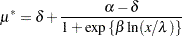 |
for , treating  as the new parameter (in lieu of ), and choosing a value for that leads to low skewness. This results in the expected-value parameterization of . Solving for yields
 |
The interpretation of the parameter that replaces in the model equation is simple: it is the mean dose response when the dose is . Fixing  , the following PROC NLIN statements fit this model:
proc nlin data=logistic bias hougaard nlinmeasures;
   parameters alpha=100 mustar=20 LD50=0.15;
   delta   = 0;
   xstar   = 0.3;
   beta    = log((alpha - mustar)/(mustar - delta)) / log(xstar/LD50);
   Switch  = 1/(1+exp(beta*log(dose/LD50)));
   model y = delta + (alpha - delta)*Switch;
   output out=nlinout pred=p lcl=lcl ucl=ucl;
run;
Note that the switch-off function continues to be written in terms of and the LD50. The only difference from the previous model is that is now expressed as a function of the parameter . Using expected-value parameterizations is a simple mechanism to lower the curvature in a model and to arrive at starting values. The starting value for can be gleaned from Output 62.4.1 at  .
.
Output 62.4.6 shows selected results from this NLIN run. The ANOVA table is again unaffected by the change in parameterization. The skewness for is significantly reduced in comparison to those of the parameter in the previous model (compare Output 62.4.6 and Output 62.4.5), while its bias remains on the same scale from Output 62.4.5 to Output 62.4.6. Also note the substantial reduction in the parameter-effects curvature values. As expected, the intrinsic curvature values remain intact.
| NOTE: Convergence criterion met. |
| Note: | An intercept was not specified for this model. |
| Source | DF | Sum of Squares | Mean Square | F Value | Approx Pr > F |
|---|---|---|---|---|---|
| Model | 3 | 33965.4 | 11321.8 | 745.50 | <.0001 |
| Error | 4 | 60.7475 | 15.1869 | ||
| Uncorrected Total | 7 | 34026.1 |
| Parameter | Estimate | Approx Std Error |
Approximate 95% Confidence Limits |
Skewness | Bias | Percent Bias |
|
|---|---|---|---|---|---|---|---|
| alpha | 101.8 | 3.0034 | 93.4752 | 110.2 | 0.1415 | 0.1512 | 0.15 |
| mustar | 20.7073 | 2.6430 | 13.3693 | 28.0454 | -0.0572 | -0.0983 | -0.47 |
| LD50 | 0.1681 | 0.00915 | 0.1427 | 0.1935 | -0.0605 | -0.00013 | -0.08 |
| Global Nonlinearity Measures | |
|---|---|
| Max Intrinsic Curvature | 0.2397 |
| RMS Intrinsic Curvature | 0.1154 |
| Max Parameter-Effects Curvature | 0.2925 |
| RMS Parameter-Effects Curvature | 0.1500 |
| Curvature Critical Value | 0.3895 |
| Raw Residual Variance | 15.187 |
| Projected Residual Variance | 5.9219 |