The NLIN Procedure
- Overview
-
Getting Started

-
Syntax
-
Details
Automatic Derivatives Measures of Nonlinearity and Diagnostics Missing Values Special Variables Troubleshooting Computational Methods Output Data Sets Confidence Intervals Covariance Matrix of Parameter Estimates Convergence Measures Displayed Output Incompatibilities with SAS 6.11 and Earlier Versions of PROC NLIN ODS Table Names ODS Graphics
-
Examples
- References
| Estimating the Parameters in the Nonlinear Model |
As an example of a nonlinear regression analysis, consider the following theoretical model of enzyme kinetics. The model relates the initial velocity of an enzymatic reaction to the substrate concentration.
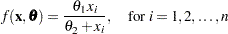 |
where  represents the amount of substrate for
  trials and
  is the velocity of the reaction. The vector
  contains the rate parameters. This model is known as the Michaelis-Menten model in biochemistry (Ratkowsky, 1990, p. 59). The model exists in many parameterizations. In the form shown here,
  is the maximum velocity of the reaction that is theoretically attainable. The parameter
  is the substrate concentration at which the velocity is 50% of the maximum.
Suppose that you want to study the relationship between concentration and velocity for a particular enzyme/substrate pair. You record the reaction rate (velocity) observed at different substrate concentrations. A SAS data set is created for this experiment in the following DATA step:
data Enzyme;
   input Concentration Velocity @@;
   datalines;
0.26 124.7   0.30 126.9
0.48 135.9   0.50 137.6
0.54 139.6   0.68 141.1
0.82 142.8   1.14 147.6
1.28 149.8   1.38 149.4
1.80 153.9   2.30 152.5
2.44 154.5   2.48 154.7
;
The SAS data set Enzyme contains the two variables Concentration (substrate concentration) and Velocity (reaction rate). The following statements fit the Michaelis-Menten model by nonlinear least squares:
proc nlin data=Enzyme method=marquardt hougaard;
   parms theta1=155
         theta2=0 to 0.07 by 0.01;
   model Velocity = theta1*Concentration / (theta2 + Concentration);
run;
The DATA= option specifies that the SAS data set Enzyme be used in the analysis. The METHOD= option directs PROC NLIN to use the MARQUARDT iterative method. The HOUGAARD option requests that a skewness measure be calculated for the parameters.
The PARMS statement declares the parameters and specifies their initial values. Suppose that  represents the velocity and
  represents the substrate concentration. In this example, the initial estimates listed in the PARMS statement for and are obtained as follows:
-
:
-
Because the model is a monotonic increasing function in
, and because 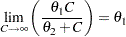
you can take the largest observed value of the variable Velocity (154.7) as the initial value for the parameter Theta1. Thus, the PARMS statement specifies 155 as the initial value for Theta1, which is approximately equal to the maximum observed velocity.
-
:
-
To obtain an initial value for the parameter
, first rearrange the model equation to solve for : 
By substituting the initial value of Theta1 for
and taking each pair of observed values of Concentration and Velocity for and , respectively, you obtain a set of possible starting values for Theta2 ranging from about 0.01 to 0.07.
You can choose any value within this range as a starting value for Theta2, or you can direct PROC NLIN to perform a preliminary search for the best initial Theta2 value within that range of values. The PARMS statement specifies a range of values for Theta2, resulting in a search over the grid points from 0 to 0.07 in increments of 0.01.
The MODEL statement specifies the enzymatic reaction model
 |
in terms of the data set variables Velocity and Concentration and in terms of the parameters in the PARMS statement.
The results from this PROC NLIN invocation are displayed in the following figures.
PROC NLIN evaluates the model at each point on the specified grid for the Theta2 parameter. Figure 62.1 displays the calculations resulting from the grid search.
| Grid Search | ||
|---|---|---|
| theta1 | theta2 | Sum of Squares |
| 155.0 | 0 | 3075.4 |
| 155.0 | 0.0100 | 2074.1 |
| 155.0 | 0.0200 | 1310.3 |
| 155.0 | 0.0300 | 752.0 |
| 155.0 | 0.0400 | 371.9 |
| 155.0 | 0.0500 | 147.2 |
| 155.0 | 0.0600 | 58.1130 |
| 155.0 | 0.0700 | 87.9662 |
The parameter Theta1 is held constant at its specified initial value of 155, the grid is traversed, and the residual sum of squares is computed at each point. The "best" starting value is the point that corresponds to the smallest value of the residual sum of squares. The best set of starting values is obtained for  (Figure 62.1). PROC NLIN uses this point from which to start the following, iterative phase of nonlinear least-squares estimation.
Figure 62.2 displays the iteration history. Note that the first entry in the "Iterative Phase" table echoes the starting values and the residual sum of squares for the best value combination in Figure 62.1. The subsequent rows of the table show the updates of the parameter estimates and the improvement (decrease) in the residual sum of squares. For this data-and-model combination, the first iteration yielded a large improvement in the sum of squares (from  to
to  ). Further steps were necessary to improve the estimates in order to achieve the convergence criterion. The NLIN procedure by default determines convergence by using R, the relative offset measure of Bates and Watts (1981). Convergence is declared when this measure is less than
  —in this example, after three iterations.
| Iterative Phase | |||
|---|---|---|---|
| Iter | theta1 | theta2 | Sum of Squares |
| 0 | 155.0 | 0.0600 | 58.1130 |
| 1 | 158.0 | 0.0736 | 19.7017 |
| 2 | 158.1 | 0.0741 | 19.6606 |
| 3 | 158.1 | 0.0741 | 19.6606 |
| NOTE: Convergence criterion met. |
| Estimation Summary | |
|---|---|
| Method | Marquardt |
| Iterations | 3 |
| R | 5.861E-6 |
| PPC(theta2) | 8.569E-7 |
| RPC(theta2) | 0.000078 |
| Object | 2.902E-7 |
| Objective | 19.66059 |
| Observations Read | 14 |
| Observations Used | 14 |
| Observations Missing | 0 |
A summary of the estimation including several convergence measures (R, PPC, RPC, and Object) is displayed in Figure 62.3.
The "R" measure in Figure 62.3 is the relative offset convergence measure of Bates and Watts. A "PPC" value of  indicates that the parameter Theta2 (which has the largest PPC value of the parameters) would change by that relative amount, if PROC NLIN were to take an additional iteration step. The "RPC" value indicates that Theta2 changed by
  , relative to its value in the last iteration. These changes are measured before step length adjustments are made. The "Object" measure indicates that the objective function changed by
  in relative value from the last iteration.
Figure 62.4 displays the analysis of variance table for the model. The table displays the degrees of freedom, sums of squares, and mean squares along with the model F test.
| Note: | An intercept was not specified for this model. |
| Source | DF | Sum of Squares | Mean Square | F Value | Approx Pr > F |
|---|---|---|---|---|---|
| Model | 2 | 290116 | 145058 | 88537.2 | <.0001 |
| Error | 12 | 19.6606 | 1.6384 | ||
| Uncorrected Total | 14 | 290135 |
| Parameter | Estimate | Approx Std Error |
Approximate 95% Confidence Limits |
Skewness | |
|---|---|---|---|---|---|
| theta1 | 158.1 | 0.6737 | 156.6 | 159.6 | 0.0152 |
| theta2 | 0.0741 | 0.00313 | 0.0673 | 0.0809 | 0.0362 |
Figure 62.5 displays the estimates for each parameter, the associated asymptotic standard error, and the upper and lower values for the asymptotic 95% confidence interval. PROC NLIN also displays the asymptotic correlations between the estimated parameters (not shown).
The skewness measures of  and
and  indicate that the parameter estimators exhibit close-to-linear behavior and that their standard errors and confidence intervals can be safely used for inferences.
Thus, the estimated nonlinear model relating reaction velocity and substrate concentration can be written as
 |
where  represents the predicted velocity or rate of the reaction, and represents the substrate concentration.