The NLIN Procedure
- Overview
-
Getting Started

-
Syntax
-
Details
Automatic Derivatives Measures of Nonlinearity and Diagnostics Missing Values Special Variables Troubleshooting Computational Methods Output Data Sets Confidence Intervals Covariance Matrix of Parameter Estimates Convergence Measures Displayed Output Incompatibilities with SAS 6.11 and Earlier Versions of PROC NLIN ODS Table Names ODS Graphics
-
Examples
- References
Example 62.1 Segmented Model
Suppose you are interested in fitting a model that consists of two segments that connect in a smooth fashion. For example, the following model states that for values of  less than
  the mean of
  is a quadratic function in , and for values of greater than the mean of is constant:
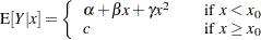 |
In this model equation  ,
,  , and
, and  are the coefficients of the quadratic segment, and
  is the plateau of the mean function. The NLIN procedure can fit such a segmented model even when the join point, , is unknown.
We also want to impose conditions on the two segments of the model. First, the curve should be continuous—that is, the quadratic and the plateau section need to meet at . Second, the curve should be smooth—that is, the first derivative of the two segments with respect to need to coincide at .
The continuity condition requires that
 |
The smoothness condition requires that
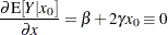 |
If you solve for and substitute into the expression for , the two conditions jointly imply that
 |
 |
|||
 |
 |
Although there are apparently four unknowns, the model contains only three parameters. The continuity and smoothness restrictions together completely determine one parameter given the other three.
The following DATA step creates the SAS data set for this example:
data a;
   input y x @@;
   datalines;
.46 1  .47  2 .57  3 .61  4 .62  5 .68  6 .69  7
.78 8  .70  9 .74 10 .77 11 .78 12 .74 13 .80 13
.80 15 .78 16
 ;
The following PROC NLIN statements fit this segmented model:
title 'Quadratic Model with Plateau';
proc nlin data=a;
   parms alpha=.45 beta=.05 gamma=-.0025;

   x0 = -.5*beta / gamma;

   if (x < x0) then
        mean = alpha + beta*x  + gamma*x*x;
   else mean = alpha + beta*x0 + gamma*x0*x0;
   model y = mean;

   if _obs_=1 and _iter_ =.  then do;
      plateau =alpha + beta*x0 + gamma*x0*x0;
      put /  x0= plateau=  ;
   end;
   output out=b predicted=yp;
run;
The parameters of the model are , , and , respectively. They are represented in the PROC NLIN statements by the variables alpha, beta, and gamma, respectively. In order to model the two segments, a conditional statement is used that assigns the appropriate expression to the mean function depending on the value of . A PUT statement is used to print the constrained parameters every time the program is executed for the first observation. The OUTPUT statement computes predicted values for plotting and saves them to data set b.
Note that there are other ways in which you can write the conditional expressions for this model. For example, you could formulate a condition with two model statements, as follows:
proc nlin data=a;
   parms alpha=.45 beta=.05 gamma=-.0025;
   x0 = -.5*beta / gamma;
   if (x < x0) then
        model y = alpha+beta*x+gamma*x*x;
   else model y = alpha+beta*x0+gamma*x0*x0;
run;
Or you could use a single expression with a conditional evaluation, as in the following statements:
proc nlin data=a;
   parms alpha=.45 beta=.05 gamma=-.0025;
   x0 = -.5*beta / gamma;
   model y = (x <x0)*(alpha+beta*x +gamma*x*x) +
             (x>=x0)*(alpha+beta*x0+gamma*x0*x0);
run;
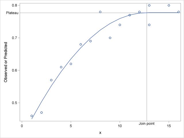
The results from fitting this model with PROC NLIN are shown in Output 62.1.1–Output 62.1.3. The iterative optimization converges after six iterations (Output 62.1.1). Output 62.1.1 indicates that the join point is  and the plateau value is
  .
.
| Quadratic Model with Plateau |
| Iterative Phase | ||||
|---|---|---|---|---|
| Iter | alpha | beta | gamma | Sum of Squares |
| 0 | 0.4500 | 0.0500 | -0.00250 | 0.0562 |
| 1 | 0.3881 | 0.0616 | -0.00234 | 0.0118 |
| 2 | 0.3930 | 0.0601 | -0.00234 | 0.0101 |
| 3 | 0.3922 | 0.0604 | -0.00237 | 0.0101 |
| 4 | 0.3921 | 0.0605 | -0.00237 | 0.0101 |
| 5 | 0.3921 | 0.0605 | -0.00237 | 0.0101 |
| 6 | 0.3921 | 0.0605 | -0.00237 | 0.0101 |
| NOTE: Convergence criterion met. |
x0=12.747669162 plateau=0.7774974276 |
| Source | DF | Sum of Squares | Mean Square | F Value | Approx Pr > F |
|---|---|---|---|---|---|
| Model | 2 | 0.1769 | 0.0884 | 114.22 | <.0001 |
| Error | 13 | 0.0101 | 0.000774 | ||
| Corrected Total | 15 | 0.1869 |
| Parameter | Estimate | Approx Std Error |
Approximate 95% Confidence Limits |
|
|---|---|---|---|---|
| alpha | 0.3921 | 0.0267 | 0.3345 | 0.4497 |
| beta | 0.0605 | 0.00842 | 0.0423 | 0.0787 |
| gamma | -0.00237 | 0.000551 | -0.00356 | -0.00118 |
The following statements produce a graph of the observed and predicted values with reference lines for the join point and plateau estimates (Output 62.1.4):
proc sgplot data=b noautolegend;
   yaxis label='Observed or Predicted';
   refline 0.777  / axis=y label="Plateau"    labelpos=min;
   refline 12.747 / axis=x label="Join point" labelpos=min;
   scatter y=y  x=x;
   series  y=yp x=x;
run;
If you want to estimate the join point directly, you can use the relationship between the parameters to change the parameterization of the model in such a way that the mean function depends directly on . Using the smoothness condition that relates to ,
 |
you can express as a function of and :
 |
Substituting for in the model equation
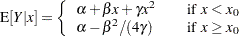 |
yields the reparameterized model
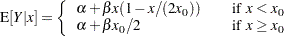 |
This model is fit with the following PROC NLIN statements:
proc nlin data=a;
   parms alpha=.45 beta=.05 x0=10;
   if (x<x0) then
        mean = alpha + beta*x *(1-x/(2*x0));
   else mean = alpha + beta*x0/2;
   model y = mean;
run;
| NOTE: Convergence criterion met. |
| Source | DF | Sum of Squares | Mean Square | F Value | Approx Pr > F |
|---|---|---|---|---|---|
| Model | 2 | 0.1769 | 0.0884 | 114.22 | <.0001 |
| Error | 13 | 0.0101 | 0.000774 | ||
| Corrected Total | 15 | 0.1869 |
| Parameter | Estimate | Approx Std Error |
Approximate 95% Confidence Limits |
|
|---|---|---|---|---|
| alpha | 0.3921 | 0.0267 | 0.3345 | 0.4497 |
| beta | 0.0605 | 0.00842 | 0.0423 | 0.0787 |
| x0 | 12.7477 | 1.2781 | 9.9864 | 15.5089 |
The analysis of variance table in the reparameterized model is the same as in the earlier analysis (compare Output 62.1.5 and Output 62.1.3). Changing the parameterization of a model does not affect the fit. The "Parameter Estimates" table now shows x0 as a parameter in the model. The estimate agrees with the earlier result that uses the PUT statement (Output 62.1.2). Since is now a model parameter, the NLIN procedure also reports its asymptotic standard error and its approximate 95% confidence interval.