PROC MODECLUS: Cluster Analysis: Hertzsprung-Russell Plot

Example 59.4 Cluster Analysis: Hertzsprung-Russell Plot

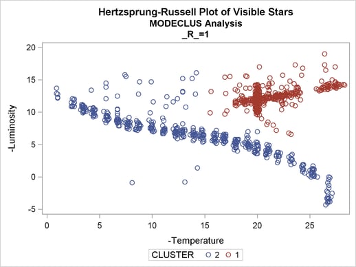
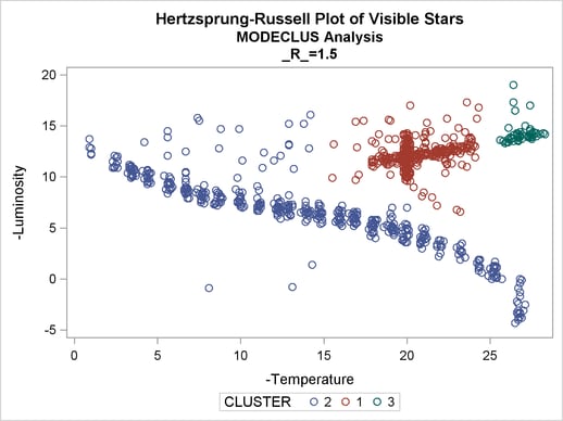
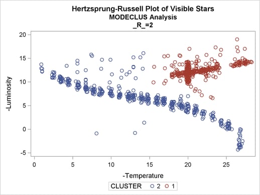
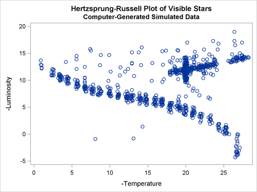
This example uses computer-generated data to mimic a Hertzsprung-Russell plot (Struve and Zebergs; 1962, p. 259) of the temperature and luminosity of stars. The data are plotted and displayed in Output 59.4.1. It appears that there are two main groups of stars and a collection of isolated stars. The long straggling group of points appearing diagonally across the figure represents the main group of stars; the more compact group in the top-right corner contains giant stars. The JOIN= option is specified at a 0.05 significance level with various smoothing parameters. The CK=5 option is specified in order to prevent the numerous outliers from forming separate clusters. The results from PROC MODECLUS is displayed in Output 59.4.2. The cluster memberships are then plotted by PROC SGPLOT, as displayed in Output 59.4.3 through Output 59.4.5.

Note that the graphic output from PROC SGPLOT in Output 59.4.3 is not available when _R_ = 2.5 because only one cluster remains after joining at a 5% significance level, and the results are not written to the OUT= data set. See the description of the JOIN= option). for more information.

The following statements produce Output 59.4.1 through Output 59.4.5:

title 'Hertzsprung-Russell Plot of Visible Stars';
title2 'Computer-Generated Simulated Data';

data hr;
   input x y @@;
   label x='-Temperature'
         y='-Luminosity';
   datalines;
1.0   12.8   0.9  13.7   0.9  12.9   1.0  12.3   1.0  12.2   2.6  10.9
2.4   10.9   2.5  11.2   2.3  11.5   2.6  12.0   2.4  12.1   2.3  10.9
2.6   11.5   2.5  11.9   2.4  11.0   3.4  11.1   3.3  11.2   3.4  11.1
3.4    9.9   3.2  10.4   3.5  10.8   3.4  11.0   3.3  11.2   3.3  10.8
3.5   10.0   3.5  10.2   3.4  10.2   3.6  10.6   3.7  10.4   3.7  10.1
3.4   10.7   3.4  10.8   3.3  11.0   3.6  10.8   3.5  10.1   4.5  10.3
4.6    9.4   4.3  10.3   4.6   9.4   4.4   9.9   4.5  10.4   4.4   9.9
4.6    9.4   4.4  10.7   4.4   9.3   4.4   9.5   4.1  10.6   4.4  10.6
4.5   10.3   4.4  10.0   4.2   9.8   4.5   9.5   4.2  13.4   4.6  10.4
4.5    9.8   5.8   8.8   5.6   8.4   5.6  13.9   5.7   9.5   5.6  14.5
5.6    9.2   5.7   8.7   5.7   9.4   5.7   9.3   5.6   9.4   5.8   9.8
5.5    8.8   5.8   8.9   5.7   9.4   5.6  12.1   5.4  10.1   5.8   9.3

   ... more lines ...   

26.4  14.1  26.6  14.2  27.5  13.7  27.6  14.4  27.8  14.0  27.4  14.7
25.8  13.5  25.6  13.6  26.8  14.4  26.4  19.0  26.0  13.4  27.3  14.0
27.5  14.3  27.4  14.5  26.3  13.8  26.9  13.7  26.3  13.7  27.7  14.3
27.3  14.1  28.3  14.2  17.4  15.5  13.8  15.2  12.0  11.6  14.1  12.8
17.1  10.2  16.9  15.4  18.5  12.6  14.2  16.1  23.2   6.6  11.4  12.4
20.4  11.7  20.9   8.1  18.9  13.7  16.9   9.7  15.5   9.9  18.3  14.2
19.3  13.7  17.0  12.9  10.1  11.6  17.9  13.5  14.3   1.4  13.1  -0.8
8.1  -0.9  20.0   7.0  21.0   8.5  15.6  13.2
;

proc sgplot data=hr;
   scatter y=y x=x;
run;

proc modeclus data=hr m=1 r=1 1.5 2 2.5 ck=5
              join=.05 short out=out;
run;

title2 'MODECLUS Analysis';

proc sgplot data=out;
   scatter y=y x=x/group=cluster;
   by _R_;
run;

Output 59.4.1 Scatter Plot of Data

Output 59.4.2 Results from PROC MODECLUS

Hertzsprung-Russell Plot of Visible Stars

Computer-Generated Simulated Data

The MODECLUS Procedure

Cluster Summary
R	CK	Number of Clusters Joined	Maximum P-value	Number of Clusters	Frequency of Unclassified Objects
1	5	14	0.0001	2	0
1.5	5	6	0.0000	3	0
2	5	4	0.0000	2	0
2.5	5	2	0.0000	1	0

Output 59.4.3 Scatter Plots of Cluster Memberships by _R_= 1

Output 59.4.4 Scatter Plots of Cluster Memberships by _R_= 1.5

Output 59.4.5 Scatter Plots of Cluster Memberships by _R_=2