The MODECLUS Procedure

Significance tests require that a fixed-radius kernel be specified for density estimation via the DR= or R= option. You can also specify the DK= or K= option, but only the fixed radius is used for the significance tests.

The purpose of the significance tests is as follows: given a simple random sample of objects from a population, obtain an estimate of the number of clusters in the population such that the probability in repeated sampling that the estimate exceeds the true number of clusters is not much greater than , 1% 10%. In other words, a sequence of null hypotheses of the form

where , is tested against the alternatives such as

with a maximum experimentwise error rate of approximately . The tests protect you from overestimating the number of population clusters. It is impossible to protect against underestimating the number of population clusters without introducing much stronger assumptions than are used here, since the number of population clusters could conceivably exceed the sample size.

The method for conducting significance tests is as follows:

1. Estimate densities by using fixed-radius uniform kernels.

2. Obtain preliminary clusters by a "valley-seeking" method. Other clustering methods could be used but would yield less power.

3. Compute an approximate p-value for each cluster by comparing the estimated maximum density in the cluster with the estimated maximum density on the cluster boundary.

4. Repeatedly join the least significant cluster with a neighboring cluster until all remaining clusters are significant.

5. Estimate the number of population clusters as the number of significant sample clusters.

6. The preceding steps can be repeated for any number of different radii, and the estimate of the number of population clusters can be taken to be the maximum number of significant sample clusters for any radius.

This method has the following useful features:

• No distributional assumptions are required.

• The choice of smoothing parameter is not critical since you can try any number of different values.

• The data can be coordinates or distances.

• Time and space requirements for the significance tests are no worse than those for obtaining the clusters.

• The power is high enough to be useful for practical purposes.

The method for computing the p-values is based on a series of plausible approximations. There are as yet no rigorous proofs that the method is infallible. Neither are there any asymptotic results. However, simulations for sample sizes ranging from 20 to 2000 indicate that the p-values are almost always conservative. The only case discovered so far in which the p-values are liberal is a uniform distribution in one dimension for which the simulated error rates exceed the nominal significance level only slightly for a limited range of sample sizes.

To make inferences regarding population clusters, it is first necessary to define what is meant by a cluster. For clustering methods that use nonparametric density estimation, a cluster is usually loosely defined as a region surrounding a local maximum of the probability density function or a maximal connected set of local maxima. This definition might not be satisfactory for very rough densities with many local maxima. It is not applicable at all to discrete distributions for which the density does not exist. As another example in which this definition is not intuitively reasonable, consider a uniform distribution in two dimensions with support in the shape of a figure eight (including the interior). This density might be considered to contain two clusters even though it does not have two distinct modes.

These difficulties can be avoided by defining clusters in terms of the local maxima of a smoothed probability density or mass function. For example, define the neighborhood distribution function (NDF) with radius r at a point x as the probability that a randomly selected point will lie within a radius r of x—that is, the probability integral over a hypersphere of radius r centered at x:

where X is the random variable being sampled, r is a user-specified radius, and d(x,y) is the distance between points x and y.

The NDF exists for all probability distributions. You can select the radius according to the degree of resolution required. The minimum-variance unbiased estimate of the NDF at a point x is proportional to the uniform-kernel density estimate with corresponding support.

You can define a modal region as a maximal connected set of local maxima of the NDF. A cluster is a connected set containing exactly one modal region. This definition seems to give intuitively reasonable results in most cases. An exception is a uniform density on the perimeter of a square. The NDF has four local maxima. There are eight local maxima along the perimeter, but running PROC MODECLUS with the R= option would yield four clusters since the two local maxima at each corner are separated by a distance equal to the radius. While this density does indeed have four distinctive features (the corners), it is not obvious that each corner should be considered a cluster.

The number of population clusters depends on the radius of the NDF. The significance tests in PROC MODECLUS protect against overestimating the number of clusters at any specified radius. It is often useful to look at the clustering results across a range of radii. A plot of the number of sample clusters as a function of the radius is a useful descriptive display, especially for high-dimensional data (Wong and Schaack; 1982).

If a population has two clusters, it must have two modal regions. If there are two modal regions, there must be a "valley" between them. It seems intuitively desirable that the boundary between the two clusters should follow the bottom of this valley. All the clustering methods in PROC MODECLUS are designed to locate the estimated cluster boundaries in this way, although methods 1 and 6 seem to be much more successful at this than the others. Regardless of the precise location of the cluster boundary, it is clear that the maximum of the NDF along the boundary between two clusters must be strictly less than the value of the NDF in either modal region; otherwise, there would be only a single modal region; according to Hartigan and Hartigan (1985), there must be a "dip" between the two modes. PROC MODECLUS assesses the significance of a sample cluster by comparing the NDF in the modal region with the maximum of the NDF along the cluster boundary. If the NDF has second-order derivatives in the region of interest and if the boundary between the two clusters is indeed at the bottom of the valley, then the maximum value of the NDF along the boundary occurs at a saddle point. Hence, this test is called a saddle test. This term is intended to describe any test for clusters that compares modal densities with saddle densities, not just the test currently implemented in the MODECLUS procedure.

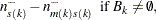
The obvious estimate of the maximum NDF in a sample cluster is the maximum estimated NDF at an observation in the cluster. Let be the index of the observation for which the maximum is attained in cluster k.

Estimating the maximum NDF on the cluster boundary is more complicated. One approach is to take the maximum NDF estimate at an observation in the cluster that has a neighbor belonging to another cluster. This method yields excessively large estimates when the neighborhood is large. Another approach is to try to choose an object closer to the boundary by taking the observation with the maximum sum of estimated densities of neighbors belonging to a different cluster. After some experimentation, it is found that a combination of these two methods works well. Let be the set of indices of observations in cluster k that have neighbors belonging to a different cluster, and compute

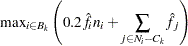Let be the index of the observation for which the maximum is attained.

Using the notation for the cardinality of set S, let

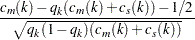
Let be a random variable distributed as the range of a random sample of u observations from a standard normal distribution. Then the approximate p-value for cluster k is

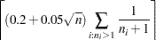
If points and are fixed a priori, would be the usual approximately normal test statistic for comparing two binomial random variables. In fact, and are selected in such a way that tends to be large and tends to be small. For this reason, and because there might be a large number of clusters, each with its own to be tested, each is referred to the distribution of instead of a standard normal distribution. If the tests are conducted for only one radius and if u is chosen equal to n, then the p-values are very conservative because (1) you are not making all possible pairwise comparisons of observations in the sample and (2) and are positively correlated if the neighborhoods overlap. In the formula for u, the summation overcorrects somewhat for the conservativeness due to correlated . The factor is empirically estimated from simulation results to adjust for the use of more than one radius.

If the JOIN option is specified, the least significant cluster (the cluster with the smallest ) is either dissolved or joined with a neighboring cluster. If no members of the cluster have neighbors belonging to a different cluster, all members of the cluster are unassigned. Otherwise, the cluster is joined to the neighboring cluster such that the sum of density estimates of neighbors of the estimated saddle point belonging to it is a maximum. Joining clusters increases the power of the saddle test. For example, consider a population with two well-separated clusters. Suppose that, for a certain radius, each population cluster is divided into two sample clusters. None of the four sample clusters is likely to be significant, but after the two sample clusters corresponding to each population cluster are joined, the remaining two clusters can be highly significant.

The saddle test implemented in PROC MODECLUS has been evaluated by simulation from known distributions. Some results are given in the following three tables. In Table 59.3, samples of 20 to 2000 observations are generated from a one-dimensional uniform distribution. For sample sizes of 1000 or less, 2000 samples are generated and analyzed by PROC MODECLUS. For a sample size of 2000, only 1000 samples are generated. The analysis is done with at least 20 different values of the R= option spread across the range of radii most likely to yield significant results. The six central columns of the table give the observed error rates at the nominal error rates at the head of each column. The standard errors of the observed error rates are given at the bottom of the table. The observed error rates are conservative for %, but they increase with and become slightly liberal for sample sizes in the middle of the range tested.

All unimodal distributions other than the uniform that have been tested, including normal, Cauchy, and exponential distributions and uniform mixtures, have produced much more conservative results. Table 59.4 displays results from a unimodal mixture of two normal distributions with equal variances and equal sampling probabilities and with means separated by two standard deviations. Any greater separation would produce a bimodal distribution. The observed error rates are quite conservative.

Table 59.4 Observed Error Rates (%) for Normal Mixture with Separation

Sample	Nominal Type 1 Error Rate						Number of
Size	1	2	5	10	15	20	Simulations
100	0.0	0.0	0.0	1.0	2.0	4.0	200
200	0.0	0.0	0.0	2.0	3.0	3.0	200
500	0.0	0.0	0.5	0.5	0.5	0.5	200

All distributions in two or more dimensions that have been tested yield extremely conservative results. For example, a uniform distribution on a circle yields observed error rates that are never more than one-tenth of the nominal error rates for sample sizes up to 1000. This conservatism is due to the fact that, as the dimensionality increases, more and more of the probability lies in the tails of the distribution (Silverman; 1986, p. 92), and the saddle test used by PROC MODECLUS is more conservative for distributions with pronounced tails. This applies even to a uniform distribution on a hypersphere because, although the density does not have tails, the NDF does.

Since the formulas for the significance tests do not involve the dimensionality, no problems are created when the data are linearly dependent. Simulations of data in nonlinear subspaces (the circumference of a circle or surface of a sphere) have also yielded conservative results.

Table 59.5 displays results in terms of power for identifying two clusters in samples from a bimodal mixture of two normal distributions with equal variances and equal sampling probabilities separated by four standard deviations. In this simulation, PROC MODECLUS never indicated more than two significant clusters.

Table 59.5 Power (%) for Normal Mixture with Separation

Sample	Nominal Type 1 Error Rate						Number of
Size	1	2	5	10	15	20	Simulations
20	0.0	0.0	0.0	2.0	37.5	68.5	200
35	0.0	13.5	38.5	48.5	64.0	75.5	200
50	17.5	26.0	51.5	67.0	78.5	84.0	200
75	25.5	36.0	58.5	77.5	85.5	89.5	200
100	40.0	54.5	72.5	84.5	91.5	92.5	200
150	70.5	80.0	92.0	97.0	100.0	100.0	200
200	89.0	96.0	99.5	100.0	100.0	100.0	200

The saddle test is not as efficient as excess-mass tests for multimodality (Müller and Sawitzki; 1991; Polonik; 1993). However, there is not yet a general approximation for the distribution of excess-mass statistics to circumvent the need for simulations to do significance tests. See Minnotte (1992) for a review of tests for multimodality.