The MODECLUS Procedure

Getting Started: MODECLUS Procedure
This section illustrates how PROC MODECLUS can be used to examine the clusters of data in the following artificial data set.
data example;
   input x y @@;
   datalines;
18 18  20 22  21 20  12 23  17 12  23 25  25 20  16 27
20 13  28 22  80 20  75 19  77 23  81 26  55 21  64 24
72 26  70 35  75 30  78 42  18 52  27 57  41 61  48 64
59 72  69 72  80 80  31 53  51 69  72 81
;
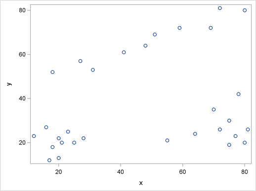
It is a good practice to plot the data to check for obvious clusters or pathologies prior to the analysis. In this example, with only two variables and a small sample size, the SGPLOT procedure in the following statements produces a scatter plot:
proc sgplot;
   scatter y=y x=x;
run;
Figure 59.1 suggests three clusters. Of these clusters, the one in the lower-left corner is the most compact, while the lower-right cluster is more dispersed.
The upper cluster is elongated and would be difficult for most clustering algorithms to identify as a single cluster. The plot also suggests that a Euclidean distance of 10 or 20 is a good initial guess for the neighborhood size in density estimation and clustering.
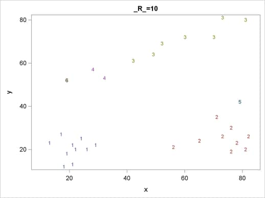
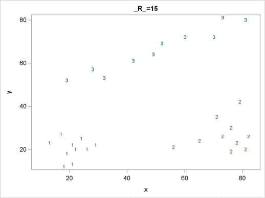
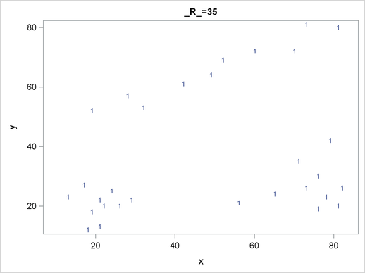
To obtain a cluster analysis in PROC MODECLUS, you must specify the METHOD= option; for most purposes, METHOD=1 is recommended. The cluster analysis can be performed with a list of radii (R=10 15 35), as shown in the following PROC MODECLUS statement. An output data set containing the cluster membership is created with the OUT= option. The following statements produce Figure 59.2 through Figure 59.5:
proc modeclus data=example method=1 r=10 15 35 out=out;
run;
For each cluster solution, PROC MODECLUS produces a table of cluster statistics including the cluster number, the number of observations in the cluster, the maximum estimated density within the cluster, the number of observations in the cluster having a neighbor that belongs to a different cluster, and the estimated saddle density of the cluster. The results are displayed in Figure 59.2, Figure 59.3, and Figure 59.4 for three different radii. A smaller radius (R=10) yields a larger number of clusters (6), as displayed in Figure 59.2; a larger radius (R=35) includes all observations in a single cluster, as displayed in Figure 59.4. Note that all clusters in these three figures are "isolated" since their corresponding boundary frequencies are all zeros. Consequently, all the estimated saddle densities are missing. A table summarizing each cluster solution is then produced at the end, as displayed in Figure 59.5.
| Cluster Statistics | ||||
|---|---|---|---|---|
| Cluster | Frequency | Maximum Estimated Density |
Boundary Frequency |
Estimated Saddle Density |
| 1 | 10 | 0.00106103 | 0 | . |
| 2 | 9 | 0.00084883 | 0 | . |
| 3 | 7 | 0.00031831 | 0 | . |
| 4 | 2 | 0.00021221 | 0 | . |
| 5 | 1 | 0.0001061 | 0 | . |
| 6 | 1 | 0.0001061 | 0 | . |
| Cluster Statistics | ||||
|---|---|---|---|---|
| Cluster | Frequency | Maximum Estimated Density |
Boundary Frequency |
Estimated Saddle Density |
| 1 | 10 | 0.00047157 | 0 | . |
| 2 | 10 | 0.00042441 | 0 | . |
| 3 | 10 | 0.00023579 | 0 | . |
| Cluster Statistics | ||||
|---|---|---|---|---|
| Cluster | Frequency | Maximum Estimated Density |
Boundary Frequency |
Estimated Saddle Density |
| 1 | 30 | 0.00012126 | 0 | . |
| Cluster Summary | ||
|---|---|---|
| R | Number of Clusters |
Frequency of Unclassified Objects |
| 10 | 6 | 0 |
| 15 | 3 | 0 |
| 35 | 1 | 0 |
The OUT= data set contains a complete copy of the input data set for each cluster solution. By using a BY statement in the following PROC SGPLOT statement, you can examine the differences in cluster memberships for each radius as shown in Figure 59.6 through Figure 59.8:
proc sgplot data=out noautolegend;
   scatter y=y x=x / group=cluster markerchar=cluster;
   by _r_;
run;