The HPQUANTSELECT Procedure

This example is modeled on the example in the section Getting Started: QUANTSELECT Procedure in SAS/STAT 14.1 User's Guide. It highlights the use of the HPQUANTSELECT procedure for multiple-level quantile regression by creating growth charts for men’s body mass index (BMI).

BMI, which is defined as the ratio of weight (kg) to squared height (m), is a standard measure for categorizing individuals as overweight or underweight. The percentiles of BMI for specified ages are of particular interest. This example draws smooth BMI quantile curves conditional on Age, which can serve as BMI growth charts in medical diagnosis to identify BMI percentiles for subjects.

The BMIMen data set is from the 1999–2000 and 2001–2002 survey results for men that are published by the National Center for Health Statistics. It contains the two variables BMI and Age with 3,264 observations.

data bmimen;
   input BMI Age @@;
   SqrtAge = sqrt(Age);
   InveAge = 1/Age;
   LogBMI  = log(BMI);
   datalines;
18.6  2.0 17.1  2.0 19.0  2.0 16.8  2.0 19.0  2.1  15.5   2.1
16.7  2.1 16.1  2.1 18.0  2.1 17.8  2.1 18.3  2.1  16.9   2.1
15.9  2.1 20.6  2.1 16.7  2.1 15.4  2.1 15.9  2.1  17.7   2.1

   ... more lines ...   

29.0 80.0 24.1 80.0 26.6 80.0 24.2 80.0 22.7 80.0  28.4  80.0
26.3 80.0 25.6 80.0 24.8 80.0 28.6 80.0 25.7 80.0  25.8  80.0
22.5 80.0 25.1 80.0 27.0 80.0 27.9 80.0 28.5 80.0  21.7  80.0
33.5 80.0 26.1 80.0 28.4 80.0 22.7 80.0 28.0 80.0  42.7  80.0
;

The logarithm of BMI is used as the response. (Although this approach does not improve the quantile regression fit, it helps with statistical inference.) The following statements fit quantile regression models for the BMIMen data set at 10 quantile levels:

%let quantile=0.03 0.05 0.1 0.25 0.5 0.75 0.85 0.90 0.95 0.97;
%let nq=10;

proc hpquantselect data=BMIMen;
   model logBMI = InveAge SqrtAge Age SqrtAge*Age Age*Age Age*Age*Age
         / quantile=&quantile;
   code file='bmicode.sas';
   output out=Bmiout copyvars=(BMI Age) pred=P_LogBMI;
run;

The CODE statement enables you to write a SAS DATA step to compute quantile predictions of the fitted model. The OUTPUT statement outputs the mean predicted quantiles for the 10 specified quantile levels. The PRED= option in the OUTPUT statement specifies the variable names for the quantile predictions. For examples, p1 is for quantile level 0.03, and p2 is for quantile level 0.05.

The following statements define and apply a SAS macro function to create a quantile curves plot for the BMIMen data set:

%let BMIcolor=red olive orange blue brown gray violet black gold green;

%macro plotBMI;
   data BmiPred;
      set Bmiout;
      %do j=1 %to &nq;
         predBMI&j = exp(P_LogBMI&j);
      %end;
      label %do j=1 %to &nq;
               predBMI&j=%qscan(&quantile,&j,%str( ))
            %end;;
   run;

   proc sort data=BmiPred;
      by Age;
   run;

   proc sgplot data=BmiPred;
      %do j=1 %to &nq;
         series y=predBMI&j x=Age/lineattrs=(thickness=2
         color=%qscan(&BMIcolor,&j,%str( )));
      %end;
      scatter y=BMI x=Age/markerattrs=(size=5);
   run;
%mend;

%plotBMI;

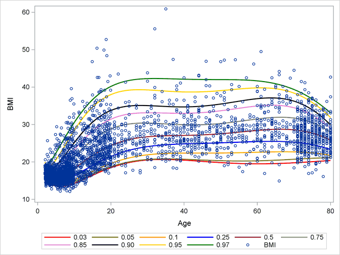
Output 14.2.1 shows the BMI quantile curves, which can serve as BMI growth charts. For example, the percentiles of any observations (small blue circles) that are located between the top 0.95 quantile (gold) curve and the 0.97 quantile (green) curve are between the 95th percentile and the 97th percentile. By using this rule, you can measure the percentile range for any observations of interest.

Other than using the OUTPUT statement, you can also calculate quantile predictions by using the CODE statement. The following statements show how to use the SAS DATA step and the SAS file bmicode, which the CODE statement requests, to calculate quantile predictions for the BMIMen data set:

data Newmen;
   set BMIMen;
   %inc bmicode;
run;

The SET statement in the SAS DATA step specifies a data set for computing quantile predictions. This is usually a new data set that you want to score. This example uses the BMIMen data set again, so the quantile predictions in the Newmen data set are identical to those in the Bmiout data set. The following statements compare the Bmiout data set with the Newmen data set:

proc compare data=Bmiout compare=Newmen criterion=0.00001;
run;