Exploring Data in Two Dimensions

Line Plots

Line plots are often used to show trends over time. For example, you can explore the patterns in pollutant concentrations in the AIR data set by following these steps.

Open the AIR data set.

This data set contains measurements of air quality as indicated by concentrations of various pollutants. Among the pollutants are carbon monoxide (CO), ozone (O3), sulfur dioxide (SO2), nitrogen oxide (NO), and DUST.

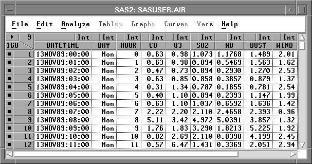
Figure 5.18: AIR Data

Choose Analyze:Line Plot ( Y X ).

This displays the line plot variables dialog.

[menu]

Figure 5.19: Creating a Line Plot

Assign CO and SO2 the Y role, and DATETIME the X role.

Assign DATETIME the Label role also. Then click OK.

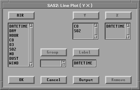
Figure 5.20: Assigning Line Plot Variables

This creates a line plot with one line for each Y variable.

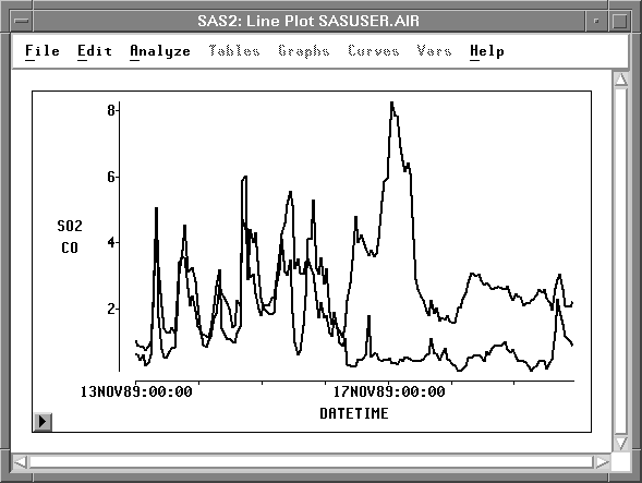
Figure 5.21: Line Plot

To associate lines with variables, simply select the variable.

Click on the SO2 variable.

This highlights both the variable and the corresponding line.

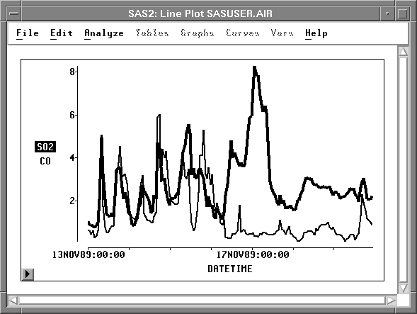
Figure 5.22: SO2 Selected

By clicking on the variables, you can see that the SO2 concentration rises to a peak on the 17th of November and then falls. The CO concentration shows a regular pattern of peaks and valleys up until the 16th; then it falls also.

To show more information, you can add observation markers to the line plot.

Click on the menu button in the lower left corner of the plot. Choose Observations.

[menu]

Figure 5.23: Line Plot Pop-up Menu

This displays the line plot with observation markers.

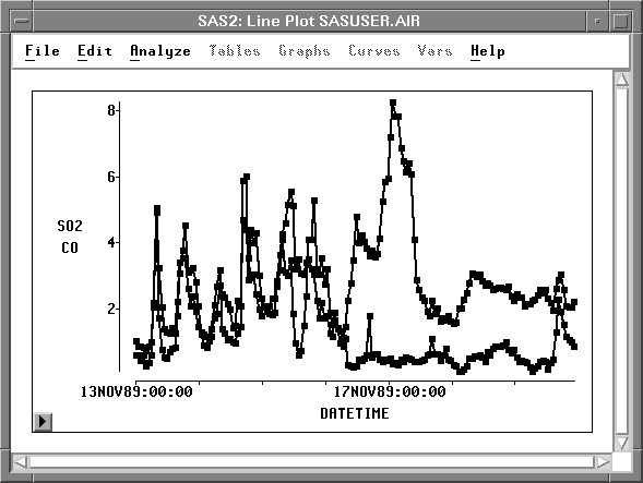
Figure 5.24: Line Plot with Observations

Point and click to identify observations with the highest pollutant concentrations.

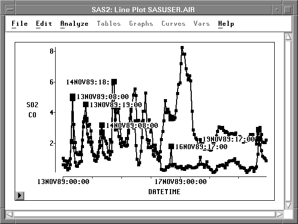
Figure 5.25: Identifying Observations

Most of the peaks for CO occur in the morning and evening, around hours 08:00 or 18:00. Carbon monoxide pollution is often caused by automobiles, so these peaks might be caused by rush-hour traffic.

The SO2 concentration follows a different pattern. Sulfur dioxide is a pollutant given off by power plants. Perhaps there was a peak demand for electricity on the 17th.

The drop in pollutants after the 17th can be partly explained by noting that the 18th and 19th were Saturday and Sunday. The weekend eliminates rush-hour traffic patterns. However, the CO level dropped on the 16th also, which was Thursday. There is an additional factor at work here.

Choose Edit:Windows:Renew to re-create the line plot.

Add WIND to the Y variable list. Then click OK.

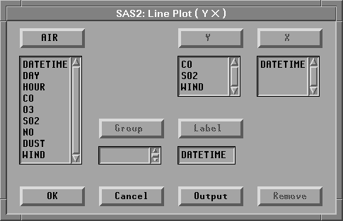
Figure 5.26: Adding WIND Variable

In the line plot, click on the WIND variable.

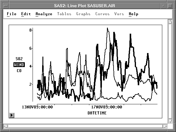
Figure 5.27: WIND Speed

Not only were the 18th and 19th a weekend, but there were high winds on the 16th, 17th, 18th, and 19th. These winds cleared much of the pollutants from the local atmosphere.