The RELIABILITY Procedure
- Overview
-
Getting Started
 Analysis of Right-Censored Data from a Single PopulationWeibull Analysis Comparing Groups of DataAnalysis of Accelerated Life Test DataWeibull Analysis of Interval Data with Common Inspection ScheduleLognormal Analysis with Arbitrary CensoringRegression ModelingRegression Model with Nonconstant ScaleRegression Model with Two Independent VariablesWeibull Probability Plot for Two Combined Failure ModesAnalysis of Recurrence Data on RepairsComparison of Two Samples of Repair DataAnalysis of Interval Age Recurrence DataAnalysis of Binomial DataThree-Parameter WeibullParametric Model for Recurrent Events DataParametric Model for Interval Recurrent Events Data
 -
SyntaxPrimary StatementsSecondary StatementsGraphical Enhancement StatementsPROC RELIABILITY StatementANALYZE StatementBY StatementCLASS StatementDISTRIBUTION StatementEFFECTPLOT StatementESTIMATE StatementFMODE StatementFREQ StatementINSET StatementLOGSCALE StatementLSMEANS StatementLSMESTIMATE StatementMAKE StatementMCFPLOT StatementMODEL StatementNENTER StatementNLOPTIONS StatementPROBPLOT StatementRELATIONPLOT StatementSLICE StatementSTORE StatementTEST StatementUNITID Statement
-
DetailsAbbreviations and NotationTypes of Lifetime DataProbability DistributionsProbability PlottingNonparametric Confidence Intervals for Cumulative Failure ProbabilitiesParameter Estimation and Confidence IntervalsRegression Model Statistics Computed for Each Observation for Lifetime DataRegression Model Statistics Computed for Each Observation for Recurrent Events DataRecurrence Data from Repairable SystemsODS Table NamesODS Graphics
- References
Weibull Analysis of Interval Data with Common Inspection Schedule
Table 17.1 shows data for 167 identical turbine parts provided by Nelson (1982, p. 415). The parts were inspected at certain times to determine which parts had cracked since the last inspection. The times at which parts develop cracks are to be fitted with a Weibull distribution.
Table 17.1: Turbine Part Cracking Data
|
Inspection (Months) |
Number |
||
|---|---|---|---|
|
Start |
End |
Cracked |
Cumulative |
|
0 |
6.12 |
5 |
5 |
|
6.12 |
19.92 |
16 |
21 |
|
19.92 |
29.64 |
12 |
33 |
|
29.64 |
35.40 |
18 |
51 |
|
35.40 |
39.72 |
18 |
69 |
|
39.72 |
45.24 |
2 |
71 |
|
45.24 |
52.32 |
6 |
77 |
|
52.32 |
63.48 |
17 |
94 |
|
63.48 |
Survived |
73 |
167 |
Table 17.1 shows the time in months of each inspection period and the number of cracked parts found in each period. These data are said to be interval censored since only the time interval in which failures occurred is known, not the exact failure times. Seventy-three parts had not cracked at the last inspection, which took place at 63.48 months. These 73 lifetimes are right censored, since the lifetimes are known only to be greater than 63.48 months.
The interval data in this example are read from a SAS data set with a special structure. All units must have a common inspection schedule. This type of interval data is called readout data. The following SAS program creates the SAS data set named CRACKS, shown in Figure 17.11, and provides the data in Table 17.1 with this structure:
data cracks;
   input Time units fail;
   datalines;
6.12  167 5
19.92 162 16
29.64 146 12
35.4  134 18
39.72 116 18
45.24 98  2
52.32 96  6
63.48 90 17
;
The variable Time is the inspection time—that is, the upper endpoint of each interval. The variable Units is the number of unfailed units at the beginning of each interval, and the variable Fail is the number of units with cracks at the inspection time.
Figure 17.11: Listing of the Turbine Part Cracking Data
The following statements use the RELIABILITY procedure to produce the probability plot in Figure 17.12 for the data in the data set CRACKS:
proc reliability data=cracks;
   freq fail;
   nenter units;
   distribution Weibull;
   probplot time / readout
                   ppout
                   pconfplt
                   noconf;
run;
The FREQ statement specifies that the variable Fail provides the number of failures in each interval. The NENTER statement specifies that the variable Units provides the number of unfailed units at the beginning of each interval. The DISTRIBUTION statement specifies that the Weibull
distribution be used for parameter estimation and probability plotting. The PROBPLOT statement requests a probability plot
of the data.
The PROBPLOT statement option READOUT indicates that the data in the CRACKS data set are readout (or interval) data. The option PCONFPLT specifies that confidence intervals for the cumulative probability of failure be plotted. The confidence intervals for the cumulative probability are based on the binomial distribution for time intervals until right censoring occurs. For time intervals after right censoring occurs, the binomial distribution is not valid, and a normal approximation is used to compute confidence intervals.
The option NOCONF suppresses the display of confidence intervals for distribution percentiles in the probability plot.
Figure 17.12: Weibull Probability Plot for the Part Cracking Data
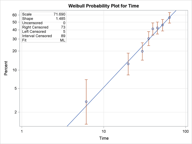
A listing of the tabular output produced by the preceding SAS statements is shown in Figure 17.13 and Figure 17.14. By default, the specified Weibull distribution is fitted by maximum likelihood. The line plotted on the probability plot and the tabular output summarize this fit. For interval data, the estimated cumulative probabilities and associated confidence intervals are tabulated. In addition, general fit information, parameter estimates, percentile estimates, standard errors, and confidence intervals are tabulated.
Figure 17.13: Partial Listing of the Tabular Output for the Part Cracking Data
| Cumulative Probability Estimates | |||||
|---|---|---|---|---|---|
| Lower Lifetime | Upper Lifetime | Cumulative Probability |
Pointwise 95% Confidence Limits |
Standard Error |
|
| Lower | Upper | ||||
| . | 6.12 | 0.0299 | 0.0125 | 0.0699 | 0.0132 |
| 6.12 | 19.92 | 0.1257 | 0.0834 | 0.1852 | 0.0257 |
| 19.92 | 29.64 | 0.1976 | 0.1440 | 0.2649 | 0.0308 |
| 29.64 | 35.4 | 0.3054 | 0.2403 | 0.3793 | 0.0356 |
| 35.4 | 39.72 | 0.4132 | 0.3410 | 0.4893 | 0.0381 |
| 39.72 | 45.24 | 0.4251 | 0.3524 | 0.5013 | 0.0383 |
| 45.24 | 52.32 | 0.4611 | 0.3869 | 0.5370 | 0.0386 |
| 52.32 | 63.48 | 0.5629 | 0.4868 | 0.6361 | 0.0384 |
Figure 17.14: Partial Listing of the Tabular Output for the Part Cracking Data
| Weibull Percentile Estimates | ||||
|---|---|---|---|---|
| Percent | Estimate | Standard Error |
Asymptotic Normal | |
| 95% Confidence Limits | ||||
| Lower | Upper | |||
| 0.1 | 0.68534385 | 0.29999861 | 0.29060848 | 1.61625083 |
| 0.2 | 1.09324674 | 0.42889777 | 0.50673224 | 2.3586193 |
| 0.5 | 2.02798319 | 0.67429625 | 1.05692279 | 3.8912169 |
| 1 | 3.23938972 | 0.93123832 | 1.84401909 | 5.69063837 |
| 2 | 5.18330703 | 1.2581604 | 3.22101028 | 8.34106988 |
| 5 | 9.70579945 | 1.78869256 | 6.76335893 | 13.9283666 |
| 10 | 15.7577991 | 2.22445157 | 11.9491109 | 20.7804776 |
| 20 | 26.1159906 | 2.6327383 | 21.4337103 | 31.821134 |
| 30 | 35.8126238 | 2.90557264 | 30.547517 | 41.9852137 |
| 40 | 45.6100472 | 3.27409792 | 39.6239146 | 52.5005271 |
| 50 | 56.0143651 | 3.89410377 | 48.8792027 | 64.1910859 |
| 60 | 67.5928125 | 4.90210777 | 58.6364803 | 77.917165 |
| 70 | 81.2334227 | 6.46932648 | 69.4938134 | 94.9562075 |
| 80 | 98.7644937 | 8.95137184 | 82.6900902 | 117.963654 |
| 90 | 125.694556 | 13.5078386 | 101.821995 | 155.164133 |
| 95 | 150.057755 | 18.2060035 | 118.300075 | 190.340791 |
| 99 | 200.437864 | 29.1957544 | 150.658574 | 266.66479 |
| 99.9 | 263.348102 | 44.7205513 | 188.791789 | 367.347666 |
In this example, the number of unfailed units at the beginning of an interval minus the number failing in the interval is equal to the number of unfailed units entering the next interval. This is not always the case since some unfailed units might be removed from the test at the end of an interval, for reasons unrelated to failure; that is, they might be right censored. The special structure of the input SAS data set required for interval data enables the RELIABILITY procedure to analyze this more general case.