The RELIABILITY Procedure
- Overview
-
Getting Started
 Analysis of Right-Censored Data from a Single PopulationWeibull Analysis Comparing Groups of DataAnalysis of Accelerated Life Test DataWeibull Analysis of Interval Data with Common Inspection ScheduleLognormal Analysis with Arbitrary CensoringRegression ModelingRegression Model with Nonconstant ScaleRegression Model with Two Independent VariablesWeibull Probability Plot for Two Combined Failure ModesAnalysis of Recurrence Data on RepairsComparison of Two Samples of Repair DataAnalysis of Interval Age Recurrence DataAnalysis of Binomial DataThree-Parameter WeibullParametric Model for Recurrent Events DataParametric Model for Interval Recurrent Events Data
 -
SyntaxPrimary StatementsSecondary StatementsGraphical Enhancement StatementsPROC RELIABILITY StatementANALYZE StatementBY StatementCLASS StatementDISTRIBUTION StatementEFFECTPLOT StatementESTIMATE StatementFMODE StatementFREQ StatementINSET StatementLOGSCALE StatementLSMEANS StatementLSMESTIMATE StatementMAKE StatementMCFPLOT StatementMODEL StatementNENTER StatementNLOPTIONS StatementPROBPLOT StatementRELATIONPLOT StatementSLICE StatementSTORE StatementTEST StatementUNITID Statement
-
DetailsAbbreviations and NotationTypes of Lifetime DataProbability DistributionsProbability PlottingNonparametric Confidence Intervals for Cumulative Failure ProbabilitiesParameter Estimation and Confidence IntervalsRegression Model Statistics Computed for Each Observation for Lifetime DataRegression Model Statistics Computed for Each Observation for Recurrent Events DataRecurrence Data from Repairable SystemsODS Table NamesODS Graphics
- References
Analysis of Right-Censored Data from a Single Population
The Weibull distribution is used in a wide variety of reliability analysis applications. This example illustrates the use of the Weibull distribution to model product life data from a single population. The following statements create a SAS data set containing observed and right-censored lifetimes of 70 diesel engine fans (Nelson 1982, p. 318):
data fan;
   input Lifetime censor @@;
   Lifetime = Lifetime/1000;
   label lifetime='Fan Life (1000s of Hours)';
   datalines;
 450 0    460 1   1150 0   1150 0   1560 1
1600 0   1660 1   1850 1   1850 1   1850 1
1850 1   1850 1   2030 1   2030 1   2030 1
2070 0   2070 0   2080 0   2200 1   3000 1
3000 1   3000 1   3000 1   3100 0   3200 1
3450 0   3750 1   3750 1   4150 1   4150 1
4150 1   4150 1   4300 1   4300 1   4300 1
4300 1   4600 0   4850 1   4850 1   4850 1
4850 1   5000 1   5000 1   5000 1   6100 1
6100 0   6100 1   6100 1   6300 1   6450 1
6450 1   6700 1   7450 1   7800 1   7800 1
8100 1   8100 1   8200 1   8500 1   8500 1
8500 1   8750 1   8750 0   8750 1   9400 1
9900 1  10100 1  10100 1  10100 1  11500 1
;
Some of the fans had not failed at the time the data were collected, and the unfailed units have right-censored lifetimes.
The variable Lifetime represents either a failure time or a censoring time in thousands of hours. The variable Censor is equal to 0 if the value of Lifetime is a failure time, and it is equal to 1 if the value is a censoring time.
If ODS Graphics is disabled, graphical output is created using traditional graphics; otherwise, ODS Graphics is used. The following statements use the RELIABILITY procedure to produce the traditional graphical output shown in Figure 17.1:
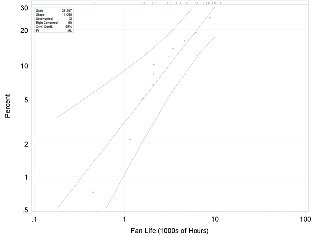
ODS Graphics OFF;
proc reliability data=fan;
   distribution Weibull;
   pplot lifetime*censor( 1 ) /  covb ;
run;
ODS Graphics ON;
The DISTRIBUTION statement specifies the Weibull distribution for probability plotting and maximum likelihood (ML) parameter
estimation. The PROBPLOT statement produces a probability plot for the variable Lifetime and specifies that the value of 1 for the variable Censor denotes censored observations. You can specify any value, or group of values, for the censor-variable (in this case, Censor) to indicate censoring times. The option COVB requests the ML parameter estimate covariance matrix.
The graphical output, displayed in Figure 17.1, consists of a probability plot of the data, an ML fitted distribution line, and confidence intervals for the percentile (lifetime) values. An inset box containing summary statistics, Weibull scale and shape estimates, and other information is displayed on the plot by default. The locations of the right-censored data values are plotted as plus signs in an area at the top of the plot.
Figure 17.1: Weibull Probability Plot for Engine Fan Data (Traditional Graphics)
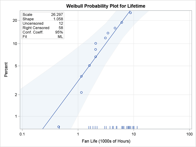
If ODS Graphics is enabled, you can create the probability plot by using ODS Graphics . The following SAS statements use ODS Graphics to create the probability plot shown in Figure 17.1:
proc reliability data=fan;
   distribution Weibull;
   pplot lifetime*censor( 1 ) /  covb;
run;
The plot is shown in Figure 17.2.
Figure 17.2: Weibull Probability Plot for Engine Fan Data (ODS Graphics)
The tabular output produced by the preceding SAS statements is shown in Figure 17.3 and Figure 17.4. This consists of summary data, fit information, parameter estimates, distribution percentile estimates, standard errors, and confidence intervals for all estimated quantities.
Figure 17.3: Tabular Output for the Fan Data Analysis
Figure 17.4: Percentile Estimates for the Fan Data
| Weibull Percentile Estimates | ||||
|---|---|---|---|---|
| Percent | Estimate | Standard Error |
Asymptotic Normal | |
| 95% Confidence Limits | ||||
| Lower | Upper | |||
| 0.1 | 0.03852697 | 0.05027782 | 0.002985 | 0.49726229 |
| 0.2 | 0.07419554 | 0.08481353 | 0.00789519 | 0.69725757 |
| 0.5 | 0.17658807 | 0.16443381 | 0.02846732 | 1.09540855 |
| 1 | 0.34072273 | 0.2635302 | 0.07482449 | 1.55152389 |
| 2 | 0.65900116 | 0.40845639 | 0.19556981 | 2.22060107 |
| 5 | 1.58925244 | 0.68465855 | 0.68311002 | 3.69738878 |
| 10 | 3.13724079 | 0.99379006 | 1.68620756 | 5.83693255 |
| 20 | 6.37467675 | 1.74261908 | 3.73051433 | 10.8930029 |
| 30 | 9.92885165 | 3.00353842 | 5.48788931 | 17.9635721 |
| 40 | 13.9407124 | 4.85766683 | 7.04177638 | 27.5986417 |
| 50 | 18.6002319 | 7.40416922 | 8.52475116 | 40.5840149 |
| 60 | 24.2121441 | 10.8733301 | 10.0408557 | 58.3842593 |
| 70 | 31.3378076 | 15.750336 | 11.7018888 | 83.9230489 |
| 80 | 41.2254517 | 23.1787018 | 13.6956839 | 124.092954 |
| 90 | 57.8253251 | 36.9266698 | 16.5405275 | 202.156081 |
| 95 | 74.1471722 | 51.6127806 | 18.9489625 | 290.137423 |
| 99 | 111.307797 | 88.1380261 | 23.5781482 | 525.462197 |
| 99.9 | 163.265082 | 144.264145 | 28.8905203 | 922.637827 |