The PARETO Procedure
- Overview
-
Getting Started

-
Syntax
-
Details
-
ExamplesCreating Before-and-After Pareto ChartsCreating Two-Way Comparative Pareto ChartsHighlighting the "Vital Few"Highlighting Combinations of CategoriesHighlighting Combinations of CellsOrdering Rows and Columns in a Comparative Pareto ChartMerging Columns in a Comparative Pareto ChartCreating Weighted Pareto ChartsCreating Alternative Pareto ChartsCustomizing Inset Labels and Formatting ValuesSpecifying Inset Headers and PositionsManaging a Large Number of Categories
- References
Example 15.2 Creating Two-Way Comparative Pareto Charts
Note: See Basic and Comparative Pareto Charts in the SAS/QC Sample Library.
During the manufacture of a MOS capacitor, different cleaning processes were used by two manufacturing systems operating in
parallel. Process A used a standard cleaning solution, and Process B used a different cleaning mixture that contained less
particulate matter. The failure causes that were observed with each process for five consecutive days were recorded and saved
in a SAS data set called Failure4:
data Failure4;
   length Process $ 9 Cause $ 16;
   label  Cause   = 'Cause of Failure';
   input  Process & $ Day & $ Cause & $ Counts;
   datalines;
Process A   March 1   Contamination    15
Process A   March 1   Corrosion         2
Process A   March 1   Doping            1
Process A   March 1   Metallization     2
Process A   March 1   Miscellaneous     3
Process A   March 1   Oxide Defect      8
Process A   March 1   Silicon Defect    1
Process A   March 2   Contamination    16
Process A   March 2   Corrosion         3
Process A   March 2   Doping            1
Process A   March 2   Metallization     3
Process A   March 2   Miscellaneous     1
Process A   March 2   Oxide Defect      9
Process A   March 2   Silicon Defect    2
Process A   March 3   Contamination    20
Process A   March 3   Corrosion         1
Process A   March 3   Doping            1
Process A   March 3   Metallization     0
Process A   March 3   Miscellaneous     3
Process A   March 3   Oxide Defect      7
Process A   March 3   Silicon Defect    2
Process A   March 4   Contamination    12
Process A   March 4   Corrosion         1
Process A   March 4   Doping            1
Process A   March 4   Metallization     0
Process A   March 4   Miscellaneous     0
Process A   March 4   Oxide Defect     10
Process A   March 4   Silicon Defect    1
Process A   March 5   Contamination    23
Process A   March 5   Corrosion         1
Process A   March 5   Doping            1
Process A   March 5   Metallization     0
Process A   March 5   Miscellaneous     1
Process A   March 5   Oxide Defect      8
Process A   March 5   Silicon Defect    2
Process B   March 1   Contamination     8
Process B   March 1   Corrosion         2
Process B   March 1   Doping            1
Process B   March 1   Metallization     4
Process B   March 1   Miscellaneous     2
Process B   March 1   Oxide Defect     10
Process B   March 1   Silicon Defect    3
Process B   March 2   Contamination     9
Process B   March 2   Corrosion         0
Process B   March 2   Doping            1
Process B   March 2   Metallization     2
Process B   March 2   Miscellaneous     4
Process B   March 2   Oxide Defect      9
Process B   March 2   Silicon Defect    2
Process B   March 3   Contamination     4
Process B   March 3   Corrosion         1
Process B   March 3   Doping            1
Process B   March 3   Metallization     0
Process B   March 3   Miscellaneous     0
Process B   March 3   Oxide Defect     10
Process B   March 3   Silicon Defect    1
Process B   March 4   Contamination     2
Process B   March 4   Corrosion         2
Process B   March 4   Doping            1
Process B   March 4   Metallization     0
Process B   March 4   Miscellaneous     3
Process B   March 4   Oxide Defect      7
Process B   March 4   Silicon Defect    1
Process B   March 5   Contamination     1
Process B   March 5   Corrosion         3
Process B   March 5   Doping            1
Process B   March 5   Metallization     0
Process B   March 5   Miscellaneous     1
Process B   March 5   Oxide Defect      8
Process B   March 5   Silicon Defect    2
;
In addition to the process variable Cause, this data set has two classification variables: Process and Day. The variable Counts is a frequency variable.
This example creates a series of displays that progressively use more of the classification information.
Basic Pareto Chart
The following statements create the first display, which analyzes the process variable without taking into account the classification variables:
title 'Pareto Analysis of Capacitor Failures';
proc pareto data=Failure4;
   vbar Cause / freq     = Counts
                last     = 'Miscellaneous'
                scale    = count
                anchor   = bl
                odstitle = title
                nlegend;
run;
The chart, shown in Output 15.2.1, indicates that contamination is the most frequently occurring problem.
Output 15.2.1: Pareto Analysis without Classification Variables
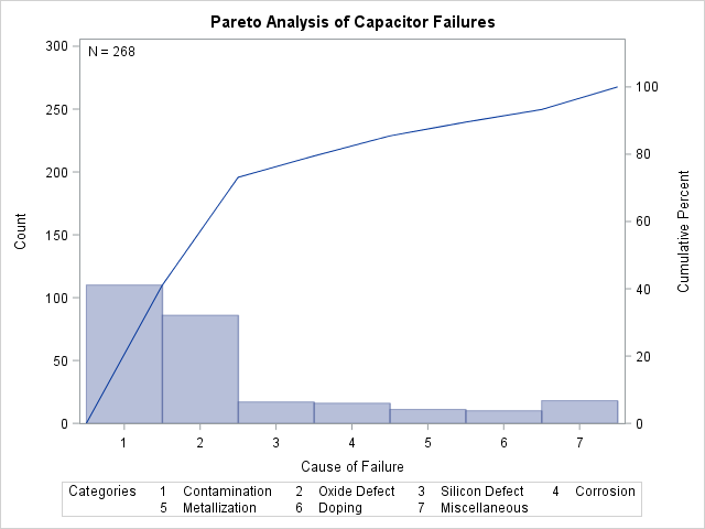
The ANCHOR= BL option anchors the cumulative percentage curve at the bottom left (BL) of the first bar. The NLEGEND option adds a sample size legend.
One-Way Comparative Pareto Chart for Process
The following statements specify Process as a classification variable to create a comparative Pareto chart, which is displayed in Output 15.2.2:
proc pareto data=Failure4;
   vbar Cause / class       = Process
                freq        = Counts
                last        = 'Miscellaneous'
                scale       = count
                odstitle    = title
                nocurve
                nlegend;
run;
Output 15.2.2: One-Way Comparative Pareto Analysis with CLASS=Process
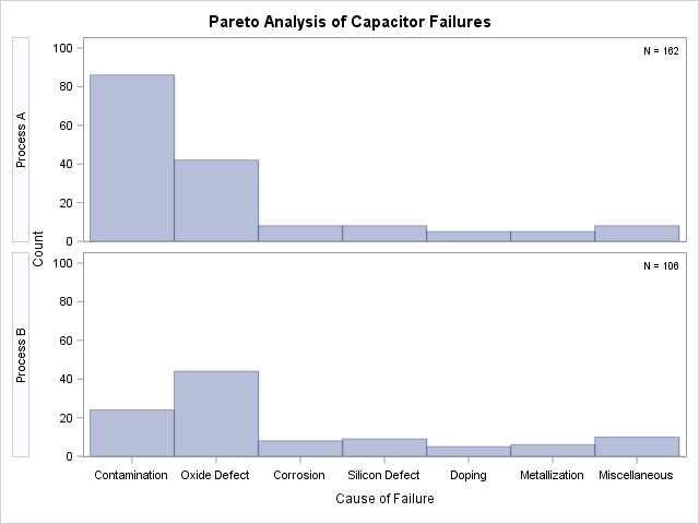
Each cell corresponds to a level of the CLASS=
variable (Process). By default, the cells are arranged from top to bottom in alphabetical order of the formatted values of Process, and the key cell is the top cell. The main difference in the two cells is a decrease in contamination when Process B is
used.
The NOCURVE option suppresses the cumulative percentage curve, along with the cumulative percentage axis.
One-Way Comparative Pareto Chart for Day
The following statements specify Day as a classification variable:
title 'Pareto Analysis by Day';
proc pareto data=Failure4;
   vbar Cause / class       = Day
                freq        = Counts
                last        = 'Miscellaneous'
                scale       = count
                catleglabel = 'Failure Causes:'
                odstitle    = title
                nrows       = 1
                ncols       = 5
                freqref     = 5 10 15 20
                nocatlabel
                nocurve
                nlegend;
run;
The NROWS= and NCOLS= options display the cells in a side-by-side arrangement. The FREQREF= option adds reference lines perpendicular to the frequency axis. The NOCATLABEL option suppresses the category axis labels, and the CATLEGLABEL= option incorporates that information into the category legend label. The chart is displayed in Output 15.2.3.
Output 15.2.3: One-Way Comparative Pareto Analysis with CLASS=Day
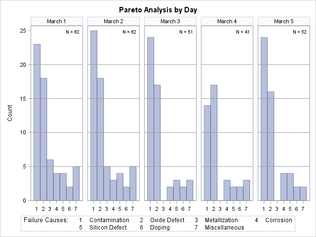
By default, the key cell is the leftmost cell. There were no failures due to metallization starting on March 3 (in fact, process controls to reduce this problem were introduced on this day).
Two-Way Comparative Pareto Chart for Process and Day
The following statements specify both Process and Day as CLASS= variables to create a two-way comparative Pareto chart:
title 'Pareto Analysis by Process and Day';
proc pareto data=Failure4;
   vbar Cause / class       = ( Process Day )
                freq        = Counts
                nrows       = 2
                ncols       = 5
                last        = 'Miscellaneous'
                scale       = count
                catleglabel = 'Failure Causes:'
                odstitle    = title
                nocatlabel
                nocurve
                nlegend;
run;
The chart is displayed in Output 15.2.4.
Output 15.2.4: Two-Way Comparative Pareto Analysis for Process and Day
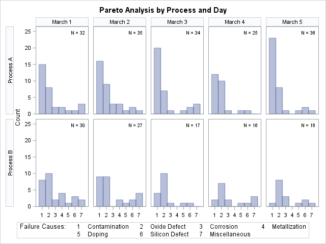
The cells are arranged in a matrix whose rows correspond to levels of the first CLASS= variable (Process) and whose columns correspond to levels of the second CLASS= variable (Day). The dimensions of the matrix are specified in the NROWS= and NCOLS= options. The key cell is in the upper left corner.
The chart reveals continuous improvement when Process B is used.