HISTOGRAM Statement: CAPABILITY Procedure

The following sections provide detailed descriptions of options specific to the HISTOGRAM statement. See Dictionary of Common Options: CAPABILITY Procedure for detailed descriptions of options common to all the plot statements.
- ALPHA=value-list
-
specifies the shape parameter
 for fitted curves requested with the BETA
, GAMMA
, PARETO
, and POWER
options. Enclose the ALPHA= option in parentheses after the distribution keyword. If you do not specify a value for , the procedure calculates a maximum likelihood estimate. See Example 5.8. You can specify A= as an alias for ALPHA= if you use it as a beta-option. You can specify SHAPE= as an alias for ALPHA= if you use it as a gamma-option.
for fitted curves requested with the BETA
, GAMMA
, PARETO
, and POWER
options. Enclose the ALPHA= option in parentheses after the distribution keyword. If you do not specify a value for , the procedure calculates a maximum likelihood estimate. See Example 5.8. You can specify A= as an alias for ALPHA= if you use it as a beta-option. You can specify SHAPE= as an alias for ALPHA= if you use it as a gamma-option.
- BARLABEL=COUNT | PERCENT | PROPORTION
-
displays labels above the histogram bars. If you specify BARLABEL=COUNT, the label shows the number of observations associated with a given bar. BARLABEL=PERCENT shows the percent of observations represented by that bar. If you specify BARLABEL=PROPORTION, the label displays the proportion of observations associated with the bar.
- BETA<(beta-options )>
-
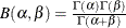
displays a fitted beta density curve on the histogram. The curve equation is
![\[ p(x) = \left\{ \begin{array}{ll} \frac{(x-\theta )^{\alpha -1}(\sigma +\theta -x)^{\beta -1}}{ B(\alpha ,\beta )\sigma ^{(\alpha +\beta -1)}} hv & \mbox{for $\theta < x < \theta + \sigma $} \\ 0 & \mbox{for $x \leq \theta $ or $x \geq \theta + \sigma $ } \end{array} \right. \]](images/qcug_capability0357.png)
where
 and
and
 lower threshold parameter (lower endpoint parameter)
  scale parameter
 shape parameter
 shape parameter
 width of histogram interval
  vertical scaling factor and
![\[ v = \left\{ \begin{array}{ll} n & \mbox{the sample size, for VSCALE=COUNT} \\ 100 & \mbox{for VSCALE=PERCENT} \\ 1 & \mbox{for VSCALE=PROPORTION} \end{array} \right. \]](images/qcug_capability0348.png)
The beta distribution is bounded below by the parameter
 and above by the value
  . You can specify and
  by using the THETA= and SIGMA= beta-options. The following statements fit a beta distribution bounded between 50 and 75 by using maximum likelihood estimates for and
  :
:
proc capability;
   histogram length / beta(theta=50 sigma=25);
run;
In general, the default values for THETA= and SIGMA= are 0 and 1, respectively. You can specify THETA=EST and SIGMA=EST to request maximum likelihood estimates for
and .
The beta distribution has two shape parameters,
and . If these parameters are known, you can specify their values with the ALPHA= and BETA= beta-options. If you do not specify values, the procedure calculates maximum likelihood estimates for and .
The BETA option can appear only once in a HISTOGRAM statement. Table 5.19 lists secondary options you can specify with the BETA option. See Example 5.8. Also see Formulas for Fitted Curves.
-
BETA=value-list
B=value-list -
specifies the second shape parameter
for beta density curves requested with the BETA option. Enclose the BETA= option in parentheses after the BETA option. If
you do not specify a value for , the procedure calculates a maximum likelihood estimate. See Example 5.8.
- BMPLOT=CARPET | DOTPLOT | SKELETAL | SCHEMATIC
-
produces a carpet plot, dot plot, or box-and-whisker plot along the bottom margin of a histogram. A carpet plot or dot plot shows the distribution of individual observations along the histogram’s horizontal axis. A carpet plot represents each observation with a vertical line. A dot plot marks each observation with a symbol. A box-and-whisker plot gives a summary of the data distribution that a histogram alone does not provide. The left and right edges of the box are located at the first and third quartiles. A central vertical line is drawn at the median and a symbol is plotted inside the box at the mean. If you specify the SKELETAL keyword, a box-and-whisker plot is produced with whiskers extending to the minimum and maximum values. If you specify SCHEMATIC, a schematic box-and-whisker plot is produced. In a schematic box-and-whisker plot, the whiskers extend to the smallest value within the lower fence and the largest value within the upper fence. Fences are defined in terms of the interquartile range (IQR). The lower fence is 1.5 IQR below the first quartile and the upper fence is 1.5 IQR above the third quartile. Each observation outside the fences is plotted with a symbol.
- C=value-list
-
specifies the shape parameter c for Weibull density curves requested with the WEIBULL option. Enclose the C= option in parentheses after the WEIBULL option. If you do not specify a value for c, the procedure calculates a maximum likelihood estimate. See Example 5.9. You can specify the SHAPE= option as an alias for the C= option.
- C=value-list | MISE
-
specifies the standardized bandwidth parameter c for kernel density estimates requested with the KERNEL option. Enclose the C= option in parentheses after the KERNEL option. You can specify up to five values to request multiple estimates. You can also specify the C=MISE option, which produces the estimate with a bandwidth that minimizes the approximate mean integrated square error (MISE). For example, the following statements compute three density estimates:
proc capability;
   histogram length / kernel(c=0.5 1.0 mise);
run;
The first two estimates have standardized bandwidths of 0.5 and 1.0, respectively, and the third has a bandwidth that minimizes the approximate MISE.
You can also use the C= option with the K= option, which specifies the kernel function, to compute multiple estimates. If you specify more kernel functions than bandwidths, the last bandwidth in the list is repeated for the remaining estimates. Likewise, if you specify more bandwidths than kernel functions, the last kernel function is repeated for the remaining estimates. For example, the following statements compute three density estimates:
proc capability;
   histogram length / kernel(c=1 2 3 k=normal quadratic);
run;
The first uses a normal kernel and a bandwidth of 1, the second uses a quadratic kernel and a bandwidth of 2, and the third uses a quadratic kernel and a bandwidth of 3. See Example 5.12.
If you do not specify a value for c, the bandwidth that minimizes the approximate MISE is used for all the estimates.
- CLIPCURVES
-
scales the vertical axis without taking fitted curves into consideration. Curves that extend above the tallest histogram bar may be clipped. You can use this option to avoid compression of the histogram bars due to extremely high fitted curve peaks.
- DELTA=value-list
-
specifies the first shape parameter
 for Johnson
  and Johnson
  density curves requested with the SB and SU options. Enclose the DELTA= option in parentheses after the SB or SU option.
If you do not specify a value for , the procedure calculates an estimate.
density curves requested with the SB and SU options. Enclose the DELTA= option in parentheses after the SB or SU option.
If you do not specify a value for , the procedure calculates an estimate.
- EDFNSAMPLES=value
-
specifies the number of simulation samples used to compute p-values for EDF goodness-of-fit statistics for density curves requested with the GUMBEL , IGAUSS , PARETO , and RAYLEIGH options. Enclose the EDFNSAMPLES= option in parentheses after the distribution option. The default value is 500.
- EDFSEED=value
-
specifies an integer value used to start the pseudo-random number generator when creating simulation samples for computing EDF goodness-of-fit statistic p-values for density curves requested with the GUMBEL , IGAUSS , PARETO , and RAYLEIGH options. Enclose the EDFSEED= option in parentheses after the distribution option. By default, the procedure uses a random number seed generated from reading the time of day from the computer’s clock.
-
ENDPOINTS
ENDPOINTS=value-list -
specifies that histogram interval endpoints, rather than midpoints, are aligned with horizontal axis tick marks. If you specify ENDPOINTS, the number of histogram intervals is based on the number of observations by using the method of Terrell and Scott (1985). If you specify ENDPOINTS=value-list, the values must be listed in increasing order and must be evenly spaced. All observations in the input data set, as well as any specification limits, must lie between the first and last values specified. The same value-list is used for all variables.
-
EXPONENTIAL<(exponential-options )>
EXP<(exponential-options )> -
displays a fitted exponential density curve on the histogram. The curve equation is
![\[ p(x) = \left\{ \begin{array}{ll} \frac{h v}{\sigma } \exp (-(\frac{x - \theta }{\sigma })) & \mbox{for $x \geq \theta $} \\ 0 & \mbox{for $x < \theta $} \end{array} \right. \]](images/qcug_capability0362.png)
where
threshold parameter scale parameter width of histogram interval vertical scaling factor and
The parameter
must be less than or equal to the minimum data value. You can specify with the THETA= exponential-option. The default value for is zero. If you specify THETA=EST, a maximum likelihood estimate is computed for . You can specify with the SIGMA= exponential-option. By default, a maximum likelihood estimate is computed for . For example, the following statements fit an exponential curve with  and with a maximum likelihood estimate for :
proc capability;
   histogram / exponential(theta=10 l=2 color=red);
run;
The curve is red and has a line type of 2. The EXPONENTIAL option can appear only once in a HISTOGRAM statement. Table 5.19 lists secondary options you can specify with the EXPONENTIAL option. See Formulas for Fitted Curves.
- FILL
-
fills areas under a parametric density curve or kernel density estimate with colors and patterns. Enclose the FILL option in parentheses after a curve option or the KERNEL option, as in the following statements:
proc capability;
   histogram length / normal(fill) cfill=green pfill=solid;
run;
Depending on the area to be filled (outside or between the specification limits), you can specify the color and pattern with options in the SPEC statement and HISTOGRAM statement, as summarized in the following table:
Area Under Curve
Statement
Option
between specification
HISTOGRAM
CFILL=
limits
HISTOGRAM
PFILL=
left of lower
SPEC
CLEFT=
specification limit
SPEC
PLEFT=
right of upper
SPEC
CRIGHT=
specification limit
SPEC
PRIGHT=
If you do not display specification limits, the CFILL= and PFILL= options specify the color and pattern for the entire area under the curve. Solid fills are used by default if patterns are not specified. You can specify the FILL option with only one fitted curve. For an example, see Output 5.8.1. Refer to SAS/GRAPH: Reference for a list of available patterns and colors. If you do not specify the FILL option but specify the options in the preceding table, the colors and patterns are applied to the corresponding areas under the histogram.
- FITINTERVAL=value
-
specifies the value of z for the method of percentiles when this method is used to fit a Johnson
or Johnson distribution. The FITINTERVAL= option is specified in parentheses after the SB
or SU
option. The default of z is 0.524.
- FITMETHOD=PERCENTILE | MLE | MOMENTS
-
specifies the method used to estimate the parameters of a Johnson
or Johnson distribution. The FITMETHOD= option is specified in parentheses after the SB
or SU
option. By default, the method of percentiles is used. You can specify the MLE keyword to request maximum likelihood estimation.
The OPTBOUNDRANGE=
, OPTMAXITER=
, OPTMAXSTARTS=
, OPTPRINT
, OPTSEED=
, and OPTTOLERANCE=
options control the optimizer that performs the maximum likelihood calculation.
- FITTOLERANCE=value
-
specifies the tolerance value for the ratio criterion when the method of percentiles is used to fit a Johnson
or Johnson distribution. The FITTOLERANCE= option is specified in parentheses after the SB
or SU
option. The default value is 0.01.
- GAMMA<(gamma-options)>
-
displays a fitted gamma density curve on the histogram. The curve equation is
![\[ p(x) = \left\{ \begin{array}{ll} \frac{h v}{\Gamma (\alpha )\sigma } (\frac{x - \theta }{\sigma })^{\alpha - 1} \exp (-(\frac{x - \theta }{\sigma })) & \mbox{for $x > \theta $} \\ 0 & \mbox{for $x \leq \theta $} \end{array} \right. \]](images/qcug_capability0363.png)
where
threshold parameter scale parameter shape parameter width of histogram interval vertical scaling factor and
The parameter
for the gamma distribution must be less than the minimum data value. You can specify with the THETA= gamma-option. The default value for is 0. If you specify THETA=EST, a maximum likelihood estimate is computed for . In addition, the gamma distribution has a shape parameter and a scale parameter . You can specify these parameters with the ALPHA= and SIGMA= gamma-options. By default, maximum likelihood estimates are computed for and . For example, the following statements fit a gamma curve with  and with maximum likelihood estimates for and :
proc capability;
   histogram length / gamma(theta=4);
run;
Note that the maximum likelihood estimate of
is calculated iteratively using the Newton-Raphson approximation. The ALPHADELTA=, ALPHAINITIAL=, and MAXITER= gamma-options control the approximation.
The GAMMA option can appear only once in a HISTOGRAM statement. Table 5.19 lists secondary options you can specify with the GAMMA option. See Example 5.9 and Formulas for Fitted Curves.
- GAMMA=value-list
-
specifies the second shape parameter
 for Johnson and Johnson density curves requested with the SB and SU options. Enclose the GAMMA= option in parentheses after the SB or SU option.
If you do not specify a value for , the procedure calculates an estimate.
for Johnson and Johnson density curves requested with the SB and SU options. Enclose the GAMMA= option in parentheses after the SB or SU option.
If you do not specify a value for , the procedure calculates an estimate.
- GRID
-
adds a grid to the histogram. Grid lines are horizontal lines positioned at major tick marks on the vertical axis.
- GUMBEL<(Gumbel-options)>
-
displays a fitted Gumbel (also known as Type 1 extreme value distribution) density curve on the histogram. The curve equation is
![\[ p(x) = \frac{h v}{\sigma }e^{-(x-\mu )/\sigma } \exp \left( -e^{-(x-\mu )/\sigma }\right) \]](images/qcug_capability0364.png)
where
 location parameter scale parameter width of histogram interval vertical scaling factor and
You can specify values for
 and with the MU=
and SIGMA=
Gumbel-options. By default, maximum likelihood estimates are computed for and .
and with the MU=
and SIGMA=
Gumbel-options. By default, maximum likelihood estimates are computed for and .
The GUMBEL option can appear only once in a HISTOGRAM statement. Table 5.19 lists secondary options you can specify with the GUMBEL option. See Formulas for Fitted Curves.
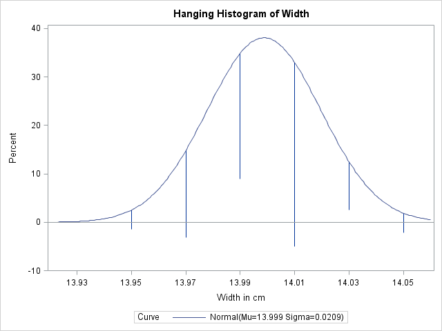
-
HANGING
HANG -
requests a hanging histogram , as illustrated in Figure 5.12.
You can use the HANGING option with only one fitted density curve. A hanging histogram aligns the tops of the histogram bars (displayed as lines) with the fitted curve. The lines are positioned at the midpoints of the histogram bins. A hanging histogram is a goodness-of-fit diagnostic in the sense that the closer the lines are to the horizontal axis, the better the fit. Hanging histograms are discussed by Tukey (1977), Wainer (1974), and Velleman and Hoaglin (1981).
- IGAUSS<(iGauss-options)>
-
displays a fitted inverse Gaussian density curve on the histogram. The curve equation is
![\[ p(x) = \left\{ \begin{array}{ll} hv \left(\frac{\lambda }{2\pi x^3}\right)^{1/2} \exp (-\frac{\lambda }{2\mu ^2 x}(x-\mu )^2) & \mbox{for $x > 0 $} \\ 0 & \mbox{for $x \leq 0 $} \end{array} \right. \]](images/qcug_capability0365.png)
where
 is the standard normal cumulative distribution function, and mean parameter
 shape parameter
  width of histogram interval vertical scaling factor and
You can specify values for
and  with the MU=
and LAMBDA=
iGauss-options. By default, the sample mean is used for and a maximum likelihood estimate is computed for .
with the MU=
and LAMBDA=
iGauss-options. By default, the sample mean is used for and a maximum likelihood estimate is computed for .
The IGAUSS option can appear only once in a HISTOGRAM statement. Table 5.19 lists secondary options you can specify with the IGAUSS option. See Formulas for Fitted Curves.
- INDICES
-
requests capability indices based on the fitted distribution. Enclose the keyword INDICES in parentheses after the distribution keyword. See Indices Using Fitted Curves for computational details and see Output 5.11.2.
- K=NORMAL | QUADRATIC | TRIANGULAR
-
specifies the kernel function (normal, quadratic, or triangular) used to compute a kernel density estimate. Enclose the K= option in parentheses after the KERNEL option, as in the following statements:
proc capability;
   histogram length / kernel(k=quadratic);
run;
You can specify kernel functions for up to five estimates. You can also use the K= option together with the C= option, which specifies standardized bandwidths. If you specify more kernel functions than bandwidths, the last bandwidth in the list is repeated for the remaining estimates. Likewise, if you specify more bandwidths than kernel functions, the last kernel function is repeated for the remaining estimates. For example, the following statements compute three estimates with bandwidths of 0.5, 1.0, and 1.5:
proc capability;
   histogram length / kernel(c=0.5 1.0 1.5 k=normal quadratic);
run;
The first estimate uses a normal kernel, and the last two estimates use a quadratic kernel. By default, a normal kernel is used.
- KERNEL<( kernel-options )>
-
superimposes up to five kernel density estimates on the histogram. You can specify the kernel-options described in the following table:
Option
Description
specifies the smoothing parameter
specifies the color of the curve
specifies that the area under the curve is to be filled
specifies the type of kernel function
specifies the line style for the curve
specifies the lower bound for the curve
specifies the character used for the kernel density curve in line printer plots
specifies the upper bound for the curve
specifies the width of the curve
You can request multiple kernel density estimates on the same histogram by specifying a list of values for either the C= or K= option. For more information, see the entries for these options. Also see Output 5.6.1 and Kernel Density Estimates. By default, kernel density estimates are computed using the AMISE method.
- LAMBDA=value
-
specifies the shape parameter
for fitted curves requested with the IGAUSS
option. Enclose the LAMBDA= option in parentheses after the IGAUSS distribution keyword. If you do not specify a value for
, the procedure calculates a maximum likelihood estimate.
- LOGNORMAL<(lognormal-options)>
-
displays a fitted lognormal density curve on the histogram. The curve equation is
![\[ p(x) = \left\{ \begin{array}{ll} \frac{h v}{\sigma \sqrt {2\pi }(x - \theta )} \exp \left(-\frac{(\log (x-\theta )-\zeta )^{2}}{2\sigma ^{2}}\right) & \mbox{for $ x > \theta $} \\ 0 & \mbox{for $ x \leq \theta $} \end{array} \right. \]](images/qcug_capability0366.png)
where
threshold parameter  scale parameter shape parameter width of histogram interval vertical scaling factor and
Note that the lognormal distribution is also referred to as the
 distribution in the Johnson system of distributions.
The parameter
for the lognormal distribution must be less than the minimum data value. You can specify with the THETA= lognormal-option. The default value for is zero. If you specify THETA=EST, a maximum likelihood estimate is computed for . You can specify the parameters and  with the SIGMA= and ZETA= lognormal-options. By default, maximum likelihood estimates are computed for and . For example, the following statements fit a lognormal distribution function with a default value of
  and with maximum likelihood estimates for and :
proc capability;
   histogram length / lognormal;
run;
The LOGNORMAL option can appear only once in a HISTOGRAM statement. Table 5.19 lists secondary options that you can specify with the LOGNORMAL option. See Example 5.9 and Formulas for Fitted Curves.
- LOWER=value-list
-
specifies lower bounds for kernel density estimates requested with the KERNEL option. Enclose the LOWER= option in parentheses after the KERNEL option. You can specify up to five lower bounds for multiple kernel density estimates. If you specify more kernel estimates than lower bounds, the last lower bound is repeated for the remaining estimates.
- MAXNBIN=n
-
specifies the maximum number of bins to be displayed in a comparative histogram. This option is useful in situations where the scales or ranges of the data distributions differ greatly from cell to cell. By default, the bin size and midpoints are determined for the key cell, and then the midpoint list is extended to accommodate the data ranges for the remaining cells. However, if the cell scales differ considerably, the resulting number of bins may be so great that each cell histogram is scaled into a narrow region. By limiting the number of bins with the MAXNBIN= option, you can narrow the window about the data distribution in the key cell. Note that the MAXNBIN= option provides an alternative to the MAXSIGMAS= option.
- MAXSIGMAS=value
-
limits the number of bins to be displayed to a range of value standard deviations (of the data in the key cell) above and below the mean of the data in the key cell. This option is useful in situations where the scales or ranges of the data distributions differ greatly from cell to cell. By default, the bin size and midpoints are determined for the key cell, and then the midpoint list is extended to accommodate the data ranges for the remaining cells. If the cell scales differ considerably, however, the resulting number of bins may be so great that each cell histogram is scaled into a narrow region. By limiting the number of bins with the MAXSIGMAS= option, you narrow the window about the data distribution in the key cell. Note that the MAXSIGMAS= option provides an alternative to the MAXNBIN= option.
- MIDPERCENTS
-
requests a table listing the midpoints and percent of observations in each histogram interval. For example, the following statements create the table in Figure 5.13:
proc capability;
   histogram Length / midpercents;
run;
If you specify the MIDPERCENTS option in parentheses after a density estimate option, a table listing the midpoints, observed percent of observations, and the estimated percent of the population in each interval (estimated from the fitted distribution) is printed.
The following statements create the table shown in Figure 5.14:
proc capability;
   histogram Length / gamma(theta=3 midpercents);
run;
- MIDPOINTS=value-list | KEY | UNIFORM
-
specifies how to determine the midpoints for the histogram intervals, where values-list determines the width of the histogram bars as the difference between consecutive midpoints. The procedure uses the same values for all variables. See Output 5.9.1.
The range of midpoints, extended at each end by half of the bar width, must cover the range of the data as well as any specification limits. For example, if you specify
midpoints=2 to 10 by 0.5
then all of the observations and specification limits should fall between 1.75 and 10.25. (Otherwise, a default list of midpoints is used.) You must use evenly spaced midpoints listed in increasing order.
- KEY
-
determines the midpoints for the data in the key cell. The initial number of midpoints is based on the number of observations in the key cell that use the method of Terrell and Scott (1985). The procedure extends the midpoint list for the key cell in either direction as necessary until it spans the data in the remaining cells.
- UNIFORM
-
determines the midpoints by using all the observations as if there were no cells. In other words, the number of midpoints is based on the total sample size by using the method of Terrell and Scott (1985).
Neither KEY nor UNIFORM apply unless you use the CLASS statement. By default, if you use a CLASS statement, MIDPOINTS=KEY. However, if the key cell is empty then MIDPOINTS=UNIFORM. Otherwise, the procedure computes the midpoints by using the algorithm described in Terrell and Scott (1985). The default midpoints are primarily applicable to continuous data that are approximately normally distributed.
If you produce traditional graphics and use the MIDPOINTS= and HAXIS= options, you can use the ORDER= option in the AXIS statement you specified with the HAXIS= option. However, for the tick mark labels to coincide with the histogram interval midpoints, the range of the ORDER= list must encompass the range of the MIDPOINTS= list, as illustrated in the following statements:
proc capability; histogram length / midpoints=20 to 80 by 10 haxis=axis1; axis1 length=6 in order=10 20 30 40 50 60 70 80 90; run; - MIDPTAXIS=name
-
is an alias for the HAXIS= option.
- MU=value-list
-
specifies the parameter
for fitted curves requested with the GUMBEL
, IGAUSS
, and NORMAL
options. Enclose the MU= option in parentheses after the distribution keyword. For the normal and inverse Gaussian distributions,
the default value of is the sample mean. If you do not specify a value for for the Gumbel distribution, the procedure calculates a maximum likelihood estimate.
- NENDPOINTS=n
-
specifies the number of histogram interval endpoints and causes the endpoints, rather than interval midpoints, to be aligned with horizontal axis tick marks.
- NMIDPOINTS=n
- NOBARS
-
suppresses drawing of histogram bars. This option is useful when you want to display fitted curves only.
-
NOCURVELEGEND
NOCURVEL -
suppresses the portion of the legend for fitted curves. If you use the INSET statement to display information about the fitted curve on the histogram, you can use the NOCURVELEGEND option to prevent the information about the fitted curve from being repeated in a legend at the bottom of the histogram. See Output 5.15.1.
- NOLEGEND
-
suppresses legends for specification limits, fitted curves, distribution lines, and hidden observations. See Example 5.13. Specifying the NOLEGEND option is equivalent to specifying LEGEND=NONE.
- NOPLOT
-
suppresses the creation of a plot. Use the NOPLOT option when you want only to print summary statistics for a fitted density or create either an OUTFIT= or an OUTHISTOGRAM= data set. See Example 5.11.
- NOPRINT
-
suppresses printed output summarizing the fitted curve. Enclose the NOPRINT option in parentheses following the distribution option. See Customizing a Histogram for an example.
- NORMAL<(normal-options)>
-
displays a fitted normal density curve on the histogram. The curve equation is
![\[ p(x) = \begin{array}{ll} \frac{h v}{\sigma \sqrt {2\pi }} \exp \left(-\frac{1}{2} (\frac{x - \mu }{\sigma })^{2}\right) & \mbox{for $-\infty < x < \infty $} \end{array} \]](images/qcug_capability0369.png)
where
mean standard deviation width of histogram interval vertical scaling factor and
Note that the normal distribution is also referred to as the
 distribution in the Johnson system of distributions.
You can specify values for
and with the MU= and SIGMA= normal-options, as shown in the following statements:
proc capability;
   histogram length / normal(mu=14 sigma=0.05);
run;
By default, the sample mean and sample standard deviation are used for
and . The NORMAL option can appear only once in a HISTOGRAM statement. Table 5.19 lists secondary options that you can specify with the NORMAL option. See Figure 5.10 and Formulas for Fitted Curves.
-
NOSPECLEGEND
NOSPECL -
suppresses the portion of the legend for specification limit reference lines. See Figure 5.11.
- NOTABCONTENTS
-
suppresses the table of contents entries for tables produced by the HISTOGRAM statement. See the section ODS Tables for descriptions of the tables produced by the HISTOGRAM statement.
- OPTBOUNDRANGE=value
-
defines the sampling range for each parameter during maximum likelihood estimation for the Johnson
distribution. PROC UNIVARIATE computes initial estimates for each parameter by using the method of percentiles. The value determines the range of parameter values around the initial estimate that can be sampled for local optimization starting
values. The default is 100.
- OPTMAXITER=value
-
limits the number of iterations that are used by the optimizer in maximum likelihood estimation for the Johnson
distribution. The default is 500.
- OPTMAXSTARTS=N
-
defines the maximum number of starting points to be used for local optimization in maximum likelihood estimation for the Johnson
distribution. That is, no more than N local optimizations are used in the multistart algorithm. The default value is 100.
- OPTPRINT
-
prints the iteration history for the Johnson
distribution maximum likelihood estimation.
- OPTSEED=value
-
specifies a positive integer seed for generating random number sequences in Johnson
distribution maximum likelihood estimation. You can use this option to replicate results from different runs.
- OPTTOLERANCE=value
-
specifies the tolerance for declaring optimality in maximum likelihood estimation for the Johnson
distribution. The default value is 1E–8.
- OUTFIT=SAS-data-set
-
creates a SAS data set that contains parameter estimates for fitted curves and related goodness-of-fit information. See Output Data Sets.
-
OUTHISTOGRAM=SAS-data-set
OUTHIST=SAS-data-set -
creates a SAS data set that contains information about histogram intervals. Specifically, the data set contains the midpoints of the histogram intervals, the observed percent of observations in each interval, and the estimated percent of observations in each interval (estimated from each of the specified fitted curves). See Output Data Sets.
- OUTKERNEL=SAS-data-set
-
creates a SAS data set containing information about kernel density estimates requested with the KERNEL option. See OUTKERNEL= Output Data Set for details.
- PARETO<(Pareto-options)>
-
displays a fitted generalized Pareto density curve on the histogram. The curve equation is
![\[ p(x) = \left\{ \begin{array}{ll} \frac{hv}{\sigma }(1 - \alpha (x-\theta )/\sigma )^{1/\alpha -1} & \mbox{if $ \alpha \neq 0$} \\ \frac{hv}{\sigma } \exp (-(x-\theta )/\sigma ) & \mbox{if $ \alpha = 0$} \end{array} \right. \]](images/qcug_capability0371.png)
where
threshold parameter scale parameter shape parameter width of histogram interval vertical scaling factor and
The parameter
must be less than the minimum data value. You can specify with the THETA=
Pareto-option. The default value for is zero. If you specify THETA=EST, a maximum likelihood estimate is computed for . In addition, the generalized Pareto distribution has a shape parameter and a scale parameter . You can specify these parameters with the ALPHA=
and SIGMA=
Pareto-options. By default, maximum likelihood estimates are computed for and .
The PARETO option can appear only once in a HISTOGRAM statement. Table 5.19 lists secondary options you can specify with the PARETO option. See Formulas for Fitted Curves.
- PCTAXIS=name|value-list
-
is an alias for the VAXIS= option.
-
PERCENTS=value-list
PERCENT=value-list -
specifies a list of percents for which quantiles calculated from the data and quantiles estimated from the fitted curve are tabulated. The percents must be between 0 and 100. Enclose the PERCENTS= option in parentheses after the curve option. The default percents are 1, 5, 10, 25, 50, 75, 90, 95, and 99.
For example, the following statements create the table shown in Figure 5.15:
proc capability;
   histogram Length / lognormal(percents=1 3 5 95 97 99);
run;
- POWER<(power-options)>
-
displays a fitted power function density curve on the histogram. The curve equation is
![\[ p(x) = \left\{ \begin{array}{ll} hv \frac{\alpha }{\sigma }\left(\frac{x-\theta }{\sigma }\right)^{\alpha -1} & \mbox{for $\theta < x < \theta + \sigma $} \\ 0 & \mbox{for $x \leq \theta $ or $x \geq \theta + \sigma $ } \end{array} \right. \]](images/qcug_capability0372.png)
where
threshold parameter scale parameter shape parameter width of histogram interval vertical scaling factor and
The parameter
must be less than or equal to the minimum data value. You can specify and with the THETA=
and the SIGMA=
power-options. The default values for and are 0 and 1, respectively. You can specify THETA=EST and SIGMA=EST to request maximum likelihood estimates for and .
In addition, the generalized Pareto distribution has a shape parameter
. You can specify with the ALPHA=
power-option. By default, a maximum likelihood estimate is computed for .
The POWER option can appear only once in a HISTOGRAM statement. Table 5.19 lists secondary options you can specify with the POWER option. See Formulas for Fitted Curves.
- RAYLEIGH<(Rayleigh-options)>
-
displays a fitted Rayleigh density curve on the histogram. The curve equation is
![\[ p(x) = \left\{ \begin{array}{ll} hv \frac{x-\theta }{\sigma ^2}e^{-(x-\theta )^2/(2\sigma ^2)} & \mbox{for $x \geq \theta $} \\ 0 & \mbox{for $x <\theta $} \end{array} \right. \]](images/qcug_capability0373.png)
where
threshold parameter scale parameter width of histogram interval vertical scaling factor and
The parameter
must be less than or equal to the minimum data value. You can specify with the THETA= Rayleigh-option. The default value for is zero. If you specify THETA=EST, a maximum likelihood estimate is computed for . You can specify with the SIGMA= Rayleigh-option. By default, a maximum likelihood estimate is computed for .
The RAYLEIGH option can appear only once in a HISTOGRAM statement. Table 5.19 lists secondary options you can specify with the RAYLEIGH option. See Formulas for Fitted Curves.
- RTINCLUDE
-
includes the right endpoint of each histogram interval in that interval. By default, the left endpoint is included in the histogram interval.
-
SB<(
 -options )>
-
displays a fitted Johnson
density curve on the histogram. The curve equation is
![\[ p(x) = \left\{ \begin{array}{ll} \frac{\delta h v}{\sigma \sqrt {2\pi } } \left[ \left( \frac{x - \theta }{\sigma } \right) \left( 1 - \frac{x - \theta }{\sigma } \right) \right]^{-1} \times & \\ \exp \left[ -\frac{1}{2} \left( \gamma + \delta \log ( \frac{x - \theta }{\theta + \sigma -x} ) \right)^2 \right] & \mbox{for $ \theta < x < \theta + \sigma $} \\ 0 & \mbox{for $ x \leq \theta $ or $ x \geq \theta + \sigma $} \end{array} \right. \]](images/qcug_capability0374.png)
where
threshold parameter  scale parameter
 shape parameter
 shape parameter
  width of histogram interval vertical scaling factor and
The
distribution is bounded below by the parameter and above by the value . The parameter must be less than the minimum data value. You can specify with the THETA= -option, or you can request that be estimated with the THETA = EST -option. The default value for is zero. The sum must be greater than the maximum data value. The default value for is one. You can specify with the SIGMA= -option, or you can request that be estimated with the SIGMA = EST -option. You can specify with the DELTA= -option, and you can specify with the GAMMA= -option. Note that the -options are given in parentheses after the SB option.
By default, the method of percentiles is used to estimate the parameters of the
distribution. Alternatively, you can request the method of moments or the method of maximum likelihood with the FITMETHOD
= MOMENTS or FITMETHOD = MLE options, respectively. Consider the following example:
proc capability;
   histogram length / sb;
   histogram length / sb( theta=est sigma=est );
   histogram length / sb( theta=0.5 sigma=8.4
                          delta=0.8 gamma=-0.6 );
run;
The first HISTOGRAM statement fits an
distribution with default values of and  and with percentile-based estimates for and . The second HISTOGRAM statement estimates all four parameters with the method of percentiles. The third HISTOGRAM statement
displays an curve with specified values for all four parameters.
and with percentile-based estimates for and . The second HISTOGRAM statement estimates all four parameters with the method of percentiles. The third HISTOGRAM statement
displays an curve with specified values for all four parameters.
The SB option can appear only once in a HISTOGRAM statement. Table 5.19 lists secondary options you can specify with the SB option.
- SIGMA=value-list
-
specifies the parameter
for fitted curves requested with the BETA
, EXPONENTIAL
, GAMMA
, GUMBEL
, LOGNORMAL
, NORMAL
, PARETO
, POWER
, RAYLEIGH
, SB
, SU
, and WEIBULL
options. Enclose the SIGMA= option in parentheses after the distribution keyword. The following table summarizes the use
of the SIGMA= option.
Distribution Keyword
SIGMA= Specifies
Default Value
Alias
scale parameter
1
SCALE=
scale parameter
maximum likelihood estimate
SCALE=
scale parameter
maximum likelihood estimate
SCALE=
scale parameter
maximum likelihood estimate
shape parameter
maximum likelihood estimate
SHAPE=
scale parameter
standard deviation
scale parameter
maximum likelihood estimate
scale parameter
1
SCALE=
scale parameter
maximum likelihood estimate
scale parameter
1
SCALE=
scale parameter
percentile-based estimate
SCALE=
scale parameter
maximum likelihood estimate
SCALE=
If you specify SIGMA=EST, an estimate is computed for
. For syntax examples, see the entries for the distribution options.
-
SU<(
 -options )>
-
displays a fitted Johnson
density curve on the histogram. The curve equation is
![\[ p(x) = \left\{ \begin{array}{ll} \frac{ \delta h v}{\sigma \sqrt {2\pi } } \frac{ 1 }{ \sqrt { 1 + \left( (x - \theta ) / \sigma \right)^2 } } \times & \\ \exp \left[ -\frac{1}{2} \left( \gamma + \delta \sinh ^{-1} \left( \frac{x - \theta }{\sigma } \right) \right)^2 \right] & \mbox{for $ x > \theta $} \\ 0 & \mbox{for $ x \leq \theta $ } \end{array} \right. \]](images/qcug_capability0381.png)
where
location parameter scale parameter shape parameter shape parameter width of histogram interval vertical scaling factor and
You can specify the parameters with the THETA=, SIGMA=, DELTA=, and GAMMA=
-options, which are enclosed in parentheses after the SU option. If you do not specify these parameters, they are estimated.
By default, the method of percentiles is used to estimate the parameters of the
distribution. Alternatively, you can request the method of moments or the method of maximum likelihood with the FITMETHOD
= MOMENTS or FITMETHOD = MLE options, respectively. Consider the following example:
proc capability;
   histogram length / su;
   histogram length / su( theta=0.5 sigma=8.4
                          delta=0.8 gamma=-0.6 );
run;
The first HISTOGRAM statement estimates all four parameters with the method of percentiles. The second HISTOGRAM statement displays an
curve with specified values for all four parameters.
The SU option can appear only once in a HISTOGRAM statement. Table 5.19 lists secondary options you can specify with the SU option.
-
THETA=value-list
THRESHOLD=value-list -
specifies the lower threshold parameter
for curves requested with the BETA
, EXPONENTIAL
, GAMMA
, LOGNORMAL
, PARETO
, POWER
, RAYLEIGH
, SB
, and WEIBULL
options, and the location parameter for curves requested with the SU
option. Enclose the THETA= option in parentheses after the curve option. See Example 5.8. The default value is zero. If you specify THETA=EST, an estimate is computed for .
- UPPER=value-list
-
specifies upper bounds for kernel density estimates requested with the KERNEL option. Enclose the UPPER= option in parentheses after the KERNEL option. You can specify up to five upper bounds for multiple kernel density estimates. If you specify more kernel estimates than upper bounds, the last upper bound is repeated for the remaining estimates.
- VSCALE=COUNT | PERCENT | PROPORTION
-
specifies the scale of the vertical axis. The value COUNT scales the data in units of the number of observations per data unit. The value PERCENT scales the data in units of percent of observations per data unit. The value PROPORTION scales the data in units of proportion of observations per data unit. See Figure 5.11 for an illustration of VSCALE=COUNT. The default is PERCENT.
- WEIBULL<(Weibull-options)>
-
displays a fitted Weibull density curve on the histogram. The curve equation is
![\[ p(x) = \left\{ \begin{array}{ll} \frac{ch v}{\sigma } (\frac{x - \theta }{\sigma })^{c - 1} \exp (-(\frac{x- \theta }{\sigma })^ c) & \mbox{for $ x > \theta $} \\ 0 & \mbox{for $ x \leq \theta $} \end{array} \right. \]](images/qcug_capability0382.png)
where
threshold parameter scale parameter  shape parameter
  width of histogram interval vertical scaling factor and
The parameter
must be less than the minimum data value. You can specify with the THETA= Weibull-option. The default value for is zero. If you specify THETA=EST, a maximum likelihood estimate is computed for . You can specify and c with the SIGMA= and C= Weibull-options. By default, maximum likelihood estimates are computed for c and . For example, the following statements fit a Weibull distribution with  and with maximum likelihood estimates for and c:
proc capability;
   histogram length / weibull(theta=15);
run;
Note that the maximum likelihood estimate of c is calculated iteratively using the Newton-Raphson approximation. The CDELTA=, CINITIAL=, and MAXITER= Weibull-options control the approximation.
The WEIBULL option can appear only once in a HISTOGRAM statement. Table 5.19 lists secondary options that you can specify with the WEIBULL option. See Example 5.9 and Formulas for Fitted Curves.
- ZETA=value-list
-
specifies a value for the scale parameter
for lognormal density curves requested with the LOGNORMAL option. Enclose the ZETA= option in parentheses after the LOGNORMAL
option. By default, the procedure calculates a maximum likelihood estimate for . You can specify the SCALE= option as an alias for the ZETA= option.