HISTOGRAM Statement: CAPABILITY Procedure

Note: See Three-Parameter Lognormal Distribution in the SAS/QC Sample Library.
If you request a lognormal fit with the LOGNORMAL option, a two-parameter lognormal distribution is assumed. This means that the shape parameter ![]() and the scale parameter
and the scale parameter ![]() are unknown (unless specified) and that the threshold
are unknown (unless specified) and that the threshold ![]() is known (it is either specified with the THETA= option or assumed to be zero).
is known (it is either specified with the THETA= option or assumed to be zero).
If it is necessary to estimate ![]() in addition to
in addition to ![]() and
and ![]() , the distribution is referred to as a three-parameter lognormal distribution. The equation for this distribution is the same as the equation given in section Lognormal Distribution but the method of maximum likelihood must be modified. This example shows how you can request a three-parameter lognormal
distribution.
, the distribution is referred to as a three-parameter lognormal distribution. The equation for this distribution is the same as the equation given in section Lognormal Distribution but the method of maximum likelihood must be modified. This example shows how you can request a three-parameter lognormal
distribution.
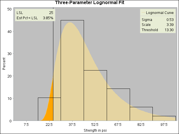
A manufacturing process (assumed to be in statistical control) produces a plastic laminate whose strength must exceed a minimum
of 25 psi. Samples are tested, and a lognormal distribution is observed for the strengths. It is important to estimate ![]() to determine whether the process is capable of meeting the strength requirement. The strengths for 49 samples are saved in
the following data set:
to determine whether the process is capable of meeting the strength requirement. The strengths for 49 samples are saved in
the following data set:
data Plastic;
   label Strength='Strength in psi';
   input Strength @@;
   datalines;
30.26 31.23 71.96 47.39 33.93 76.15 42.21
81.37 78.48 72.65 61.63 34.90 24.83 68.93
43.27 41.76 57.24 23.80 34.03 33.38 21.87
31.29 32.48 51.54 44.06 42.66 47.98 33.73
25.80 29.95 60.89 55.33 39.44 34.50 73.51
43.41 54.67 99.43 50.76 48.81 31.86 33.88
35.57 60.41 54.92 35.66 59.30 41.96 45.32
;
The following statements use the LOGNORMAL option in the HISTOGRAM statement to display the fitted three-parameter lognormal curve shown in Output 5.13.1:
ods graphics off;
title 'Three-Parameter Lognormal Fit';
proc capability data=Plastic noprint;
   spec lsl=25 cleft=orange clsl=black;
   histogram Strength / lognormal(fill color = paoy
                                       theta = est)
                        cfill  = paoy
                        cframe = ligr
                        nolegend;
   inset lsl='LSL' lslpct / cfill = ywh pos=nw;
   inset lognormal        / format=6.2 pos=ne cfill = ywh;
run;
Specifying THETA=EST requests a local maximum likelihood estimate (LMLE) for ![]() , as described by Cohen (1951). This estimate is then used to compute maximum likelihood estimates for
, as described by Cohen (1951). This estimate is then used to compute maximum likelihood estimates for ![]() and
and ![]() . The sample program CAPL3A illustrates a similar computational method implemented as a SAS/IML program.
. The sample program CAPL3A illustrates a similar computational method implemented as a SAS/IML program.
Note: See Three-Parameter Weibull Distribution in the SAS/QC Sample Library.
Note that you can specify THETA=EST as a Weibull-option to fit a three-parameter Weibull distribution.