HISTOGRAM Statement: CAPABILITY Procedure

Note: See Fitting a Beta Curve on a Histogram in the SAS/QC Sample Library.
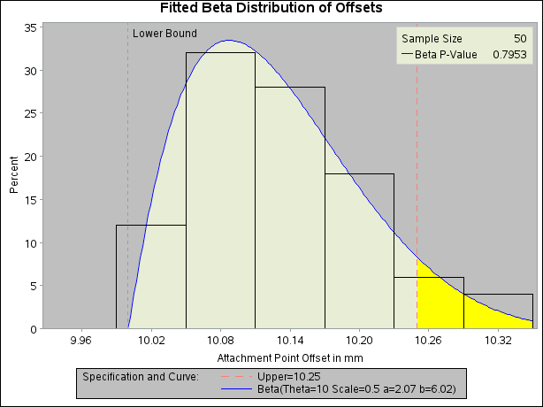
You can use a beta distribution to model the distribution of a quantity that is known to vary between lower and upper bounds. In this example, a manufacturing company uses a robotic arm to attach hinges on metal sheets. The attachment point should be offset 10.1 mm from the left edge of the sheet. The actual offset varies between 10.0 and 10.5 mm due to variation in the arm. Offsets for 50 attachment points are saved in the following data set:
data Measures;
   input Length @@;
   label Length = 'Attachment Point Offset in mm';
   datalines;
10.147 10.070 10.032 10.042 10.102
10.034 10.143 10.278 10.114 10.127
10.122 10.018 10.271 10.293 10.136
10.240 10.205 10.186 10.186 10.080
10.158 10.114 10.018 10.201 10.065
10.061 10.133 10.153 10.201 10.109
10.122 10.139 10.090 10.136 10.066
10.074 10.175 10.052 10.059 10.077
10.211 10.122 10.031 10.322 10.187
10.094 10.067 10.094 10.051 10.174
;
The following statements create a histogram with a fitted beta density curve:
ods graphics off;
legend2 frame cframe=ligr cborder=black position=center;
title1 'Fitted Beta Distribution of Offsets';
proc capability data=Measures;
   specs usl=10.25 lusl=20 cusl=salmon cright=yellow pright=solid;
   histogram Length /
      beta(theta=10 scale=0.5 color=blue fill)
      cfill     = ywh
      cframe    = ligr
      href      = 10
      hreflabel = 'Lower Bound'
      lhref     = 2
      legend    = legend2
      vaxis     = axis1;
   axis1 label=(a=90 r=0);
   inset n = 'Sample Size'
         beta(pchisq = 'P-Value') / pos=ne  cfill=ywh;
run;
The histogram is shown in Output 5.8.1. The THETA= beta-option specifies the lower threshold. The SCALE= beta-option specifies the range between the lower threshold and the upper threshold (in this case, 0.5 mm). Note that in general, the default THETA= and SCALE= values are zero and one, respectively.
The FILL beta-option specifies that the area under the curve is to be filled with the CFILL= color. (If FILL were omitted, the CFILL= color would be used to fill the histogram bars instead.) The CRIGHT= option in the SPEC statement specifies the color under the curve to the right of the upper specification limit. If the CRIGHT= option were not specified, the entire area under the curve would be filled with the CFILL= color. When a lower specification limit is available, you can use the CLEFT= option in the SPEC statement to specify the color under the curve to the left of this limit.
The HREF= option draws a reference line at the lower bound, and the HREFLABEL= option adds the label Lower Bound. The option LHREF= 2 specifies a dashed line type. The INSET statement adds an inset with the sample size and the p-value for a chi-square goodness-of-fit test.
In addition to displaying the beta curve, the BETA option summarizes the curve fit, as shown in Output 5.8.2. The output tabulates the parameters for the curve, the chi-square goodness-of-fit test whose p-value is shown in Output 5.8.1, the observed and estimated percents above the upper specification limit, and the observed and estimated quantiles. For instance, based on the beta model, the percent of offsets greater than the upper specification limit is 6.6%. For computational details, see the section Formulas for Fitted Curves.