The RELIABILITY Procedure
- Overview
-
Getting Started
 Analysis of Right-Censored Data from a Single PopulationWeibull Analysis Comparing Groups of DataAnalysis of Accelerated Life Test DataWeibull Analysis of Interval Data with Common Inspection ScheduleLognormal Analysis with Arbitrary CensoringRegression ModelingRegression Model with Nonconstant ScaleRegression Model with Two Independent VariablesWeibull Probability Plot for Two Combined Failure ModesAnalysis of Recurrence Data on RepairsComparison of Two Samples of Repair DataAnalysis of Interval Age Recurrence DataAnalysis of Binomial DataThree-Parameter WeibullParametric Model for Recurrent Events DataParametric Model for Interval Recurrent Events Data
 -
SyntaxPrimary StatementsSecondary StatementsGraphical Enhancement StatementsPROC RELIABILITY StatementANALYZE StatementBY StatementCLASS StatementDISTRIBUTION StatementEFFECTPLOT StatementESTIMATE StatementFMODE StatementFREQ StatementINSET StatementLOGSCALE StatementLSMEANS StatementLSMESTIMATE StatementMAKE StatementMCFPLOT StatementMODEL StatementNENTER StatementNLOPTIONS StatementPROBPLOT StatementRELATIONPLOT StatementSLICE StatementSTORE StatementTEST StatementUNITID Statement
-
DetailsAbbreviations and NotationTypes of Lifetime DataProbability DistributionsProbability PlottingNonparametric Confidence Intervals for Cumulative Failure ProbabilitiesParameter Estimation and Confidence IntervalsRegression Model Statistics Computed for Each Observation for Lifetime DataRegression Model Statistics Computed for Each Observation for Recurrent Events DataRecurrence Data from Repairable SystemsODS Table NamesODS Graphics
- References
Regression Modeling
This example is an illustration of a Weibull regression model that uses a load accelerated life test of rolling bearings,
with data provided by Nelson (1990, p. 305). Bearings are tested at four different loads, and lifetimes in ![]() of revolutions are measured. The data are shown in Table 16.3. An outlier identified by Nelson (1990) is omitted.
of revolutions are measured. The data are shown in Table 16.3. An outlier identified by Nelson (1990) is omitted.
Table 16.3: Bearing Lifetime Data
|
Load |
Life ( |
|||||||||
|---|---|---|---|---|---|---|---|---|---|---|
|
0.87 |
1.67 |
2.2 |
2.51 |
3.00 |
3.90 |
4.70 |
7.53 |
14.7 |
27.76 |
37.4 |
|
0.99 |
0.80 |
1.0 |
1.37 |
2.25 |
2.95 |
3.70 |
6.07 |
6.65 |
7.05 |
7.37 |
|
1.09 |
0.18 |
0.2 |
0.24 |
0.26 |
0.32 |
0.32 |
0.42 |
0.44 |
0.88 |
|
|
1.18 |
0.073 |
0.098 |
0.117 |
0.135 |
0.175 |
0.262 |
0.270 |
0.350 |
0.386 |
0.456 |
These data are modeled with a Weibull regression model in which the independent variable is the logarithm of the load. The model is
|
|
where ![]() is the location parameter of the extreme value distribution and
is the location parameter of the extreme value distribution and
|
|
for the ith bearing. The following statements create a SAS data set containing the loads, log loads, and bearing lifetimes:
data bearing;
   input load Life @@;
   lload = log(load);
   datalines;
 .87 1.67    .87 2.2    .87 2.51    .87 3.0    .87 3.9
 .87 4.7     .87 7.53   .87 14.7    .87 27.76  .87 37.4
 .99  .8     .99 1.0    .99 1.37    .99 2.25   .99 2.95
 .99 3.7     .99 6.07   .99 6.65    .99 7.05   .99 7.37
1.09  .18   1.09  .2   1.09  .24   1.09  .26  1.09  .32
1.09  .32   1.09  .42  1.09  .44   1.09  .88  1.18  .073
1.18  .098  1.18  .117 1.18  .135  1.18  .175 1.18  .262
1.18  .270  1.18  .350 1.18  .386  1.18  .456
;
Figure 16.17 shows a listing of the bearing data.
Figure 16.17: Listing of the Bearing Data
| Obs | load | Life | lload |
|---|---|---|---|
| 1 | 0.87 | 1.670 | -0.13926 |
| 2 | 0.87 | 2.200 | -0.13926 |
| 3 | 0.87 | 2.510 | -0.13926 |
| 4 | 0.87 | 3.000 | -0.13926 |
| 5 | 0.87 | 3.900 | -0.13926 |
| 6 | 0.87 | 4.700 | -0.13926 |
| 7 | 0.87 | 7.530 | -0.13926 |
| 8 | 0.87 | 14.700 | -0.13926 |
| 9 | 0.87 | 27.760 | -0.13926 |
| 10 | 0.87 | 37.400 | -0.13926 |
| 11 | 0.99 | 0.800 | -0.01005 |
| 12 | 0.99 | 1.000 | -0.01005 |
| 13 | 0.99 | 1.370 | -0.01005 |
| 14 | 0.99 | 2.250 | -0.01005 |
| 15 | 0.99 | 2.950 | -0.01005 |
| 16 | 0.99 | 3.700 | -0.01005 |
| 17 | 0.99 | 6.070 | -0.01005 |
| 18 | 0.99 | 6.650 | -0.01005 |
| 19 | 0.99 | 7.050 | -0.01005 |
| 20 | 0.99 | 7.370 | -0.01005 |
| 21 | 1.09 | 0.180 | 0.08618 |
| 22 | 1.09 | 0.200 | 0.08618 |
| 23 | 1.09 | 0.240 | 0.08618 |
| 24 | 1.09 | 0.260 | 0.08618 |
| 25 | 1.09 | 0.320 | 0.08618 |
| 26 | 1.09 | 0.320 | 0.08618 |
| 27 | 1.09 | 0.420 | 0.08618 |
| 28 | 1.09 | 0.440 | 0.08618 |
| 29 | 1.09 | 0.880 | 0.08618 |
| 30 | 1.18 | 0.073 | 0.16551 |
| 31 | 1.18 | 0.098 | 0.16551 |
| 32 | 1.18 | 0.117 | 0.16551 |
| 33 | 1.18 | 0.135 | 0.16551 |
| 34 | 1.18 | 0.175 | 0.16551 |
| 35 | 1.18 | 0.262 | 0.16551 |
| 36 | 1.18 | 0.270 | 0.16551 |
| 37 | 1.18 | 0.350 | 0.16551 |
| 38 | 1.18 | 0.386 | 0.16551 |
| 39 | 1.18 | 0.456 | 0.16551 |
The following statements fit the regression model by maximum likelihood that uses the Weibull distribution:
ods output modobstats = Residual;
proc reliability data=bearing;
   distribution Weibull;
   model life = lload /  covb
                         corrb
                         obstats
                         ;
run;
The PROC RELIABILITY statement invokes the procedure and identifies BEARING as the input data set. The DISTRIBUTION statement
specifies the Weibull distribution for model fitting. The MODEL statement specifies the regression model, identifying Life as the variable that provides the response values (the lifetimes) and Lload as the independent variable (the log loads). The MODEL statement option COVB requests the regression parameter covariance
matrix, and the CORRB option requests the correlation matrix. The option OBSTATS requests a table that contains residuals,
predicted values, and other statistics. The ODS OUTPUT statement creates a SAS data set named RESIDUAL that contains the table created by the OBSTATS option.
Figure 16.18 shows the tabular output produced by the RELIABILITY procedure. The “Weibull Parameter Estimates” table contains parameter estimates, their standard errors, and 95% confidence intervals. In this table, INTERCEPT corresponds
to ![]() , LLOAD corresponds to
, LLOAD corresponds to ![]() , and SHAPE corresponds to the Weibull shape parameter. Figure 16.19 shows a listing of the output data set
, and SHAPE corresponds to the Weibull shape parameter. Figure 16.19 shows a listing of the output data set RESIDUAL.
Figure 16.18: Analysis Results for the Bearing Data
| Model Information | |
|---|---|
| Input Data Set | WORK.BEARING |
| Analysis Variable | Life |
| Distribution | Weibull |
| Parameter Information | |
|---|---|
| Parameter | Effect |
| Prm1 | Intercept |
| Prm2 | lload |
| Prm3 | EV Scale |
| Algorithm converged. |
| Summary of Fit | |
|---|---|
| Observations Used | 39 |
| Uncensored Values | 39 |
| Maximum Loglikelihood | -51.77737 |
| Weibull Parameter Estimates | ||||
|---|---|---|---|---|
| Parameter | Estimate | Standard Error | Asymptotic Normal | |
| 95% Confidence Limits | ||||
| Lower | Upper | |||
| Intercept | 0.8323 | 0.1410 | 0.5560 | 1.1086 |
| lload | -13.8529 | 1.2333 | -16.2703 | -11.4356 |
| EV Scale | 0.8043 | 0.0999 | 0.6304 | 1.0260 |
| Weibull Shape | 1.2434 | 0.1545 | 0.9746 | 1.5862 |
| Estimated Covariance Matrix Weibull Parameters |
|||
|---|---|---|---|
| Prm1 | Prm2 | Prm3 | |
| Prm1 | 0.01987 | -0.04374 | -0.00492 |
| Prm2 | -0.04374 | 1.52113 | 0.01578 |
| Prm3 | -0.00492 | 0.01578 | 0.00999 |
| Estimated Correlation Matrix Weibull Parameters |
|||
|---|---|---|---|
| Prm1 | Prm2 | Prm3 | |
| Prm1 | 1.0000 | -0.2516 | -0.3491 |
| Prm2 | -0.2516 | 1.0000 | 0.1281 |
| Prm3 | -0.3491 | 0.1281 | 1.0000 |
Figure 16.19: Listing of Data Set Residual
| Obs | Life | lload | Xbeta | Surv | Resid | SRESID | Aresid |
|---|---|---|---|---|---|---|---|
| 1 | 1.67 | -0.139262 | 2.7614742 | 0.9407681 | -2.248651 | -2.795921 | -2.795921 |
| 2 | 2.2 | -0.139262 | 2.7614742 | 0.9175782 | -1.973017 | -2.453205 | -2.453205 |
| 3 | 2.51 | -0.139262 | 2.7614742 | 0.9036277 | -1.841191 | -2.289296 | -2.289296 |
| 4 | 3 | -0.139262 | 2.7614742 | 0.8811799 | -1.662862 | -2.067565 | -2.067565 |
| 5 | 3.9 | -0.139262 | 2.7614742 | 0.8392186 | -1.400498 | -1.741347 | -1.741347 |
| 6 | 4.7 | -0.139262 | 2.7614742 | 0.8016738 | -1.213912 | -1.50935 | -1.50935 |
| 7 | 7.53 | -0.139262 | 2.7614742 | 0.6721971 | -0.742579 | -0.923306 | -0.923306 |
| 8 | 14.7 | -0.139262 | 2.7614742 | 0.4015113 | -0.073627 | -0.091546 | -0.091546 |
| 9 | 27.76 | -0.139262 | 2.7614742 | 0.1337746 | 0.562122 | 0.6989298 | 0.6989298 |
| 10 | 37.4 | -0.139262 | 2.7614742 | 0.0542547 | 0.8601965 | 1.069549 | 1.069549 |
| 11 | 0.8 | -0.01005 | 0.971511 | 0.7973909 | -1.194655 | -1.485407 | -1.485407 |
| 12 | 1 | -0.01005 | 0.971511 | 0.741702 | -0.971511 | -1.207955 | -1.207955 |
| 13 | 1.37 | -0.01005 | 0.971511 | 0.6427726 | -0.6567 | -0.816526 | -0.816526 |
| 14 | 2.25 | -0.01005 | 0.971511 | 0.4408692 | -0.160581 | -0.199663 | -0.199663 |
| 15 | 2.95 | -0.01005 | 0.971511 | 0.3175927 | 0.1102941 | 0.1371372 | 0.1371372 |
| 16 | 3.7 | -0.01005 | 0.971511 | 0.2186832 | 0.3368218 | 0.4187966 | 0.4187966 |
| 17 | 6.07 | -0.01005 | 0.971511 | 0.0600164 | 0.8318476 | 1.0343005 | 1.0343005 |
| 18 | 6.65 | -0.01005 | 0.971511 | 0.0428027 | 0.9231058 | 1.147769 | 1.147769 |
| 19 | 7.05 | -0.01005 | 0.971511 | 0.0337583 | 0.9815166 | 1.2203956 | 1.2203956 |
| 20 | 7.37 | -0.01005 | 0.971511 | 0.0278531 | 1.0259067 | 1.2755892 | 1.2755892 |
| 21 | 0.18 | 0.0861777 | -0.361531 | 0.8303684 | -1.353268 | -1.682623 | -1.682623 |
| 22 | 0.2 | 0.0861777 | -0.361531 | 0.809042 | -1.247907 | -1.55162 | -1.55162 |
| 23 | 0.24 | 0.0861777 | -0.361531 | 0.7665749 | -1.065586 | -1.324925 | -1.324925 |
| 24 | 0.26 | 0.0861777 | -0.361531 | 0.7455451 | -0.985543 | -1.225402 | -1.225402 |
| 25 | 0.32 | 0.0861777 | -0.361531 | 0.6837688 | -0.777904 | -0.967228 | -0.967228 |
| 26 | 0.32 | 0.0861777 | -0.361531 | 0.6837688 | -0.777904 | -0.967228 | -0.967228 |
| 27 | 0.42 | 0.0861777 | -0.361531 | 0.5868036 | -0.50597 | -0.629112 | -0.629112 |
| 28 | 0.44 | 0.0861777 | -0.361531 | 0.5684693 | -0.45945 | -0.57127 | -0.57127 |
| 29 | 0.88 | 0.0861777 | -0.361531 | 0.2625812 | 0.2336973 | 0.290574 | 0.290574 |
| 30 | 0.073 | 0.1655144 | -1.460578 | 0.7887184 | -1.156718 | -1.438237 | -1.438237 |
| 31 | 0.098 | 0.1655144 | -1.460578 | 0.7101313 | -0.86221 | -1.072052 | -1.072052 |
| 32 | 0.117 | 0.1655144 | -1.460578 | 0.6526714 | -0.685003 | -0.851717 | -0.851717 |
| 33 | 0.135 | 0.1655144 | -1.460578 | 0.6006317 | -0.541902 | -0.673789 | -0.673789 |
| 34 | 0.175 | 0.1655144 | -1.460578 | 0.4946523 | -0.282391 | -0.351119 | -0.351119 |
| 35 | 0.262 | 0.1655144 | -1.460578 | 0.3126729 | 0.1211675 | 0.1506569 | 0.1506569 |
| 36 | 0.27 | 0.1655144 | -1.460578 | 0.2991233 | 0.1512449 | 0.1880546 | 0.1880546 |
| 37 | 0.35 | 0.1655144 | -1.460578 | 0.1889073 | 0.4107561 | 0.5107249 | 0.5107249 |
| 38 | 0.386 | 0.1655144 | -1.460578 | 0.1522503 | 0.5086604 | 0.6324568 | 0.6324568 |
| 39 | 0.456 | 0.1655144 | -1.460578 | 0.0987061 | 0.6753158 | 0.8396724 | 0.8396724 |
The value of the lifetime Life and the log load Lload are included in this data set, as well as statistics computed from the fitted model. The variable Xbeta is the value of the linear predictor
|
|
for each observation. The variable Surv contains the value of the reliability function, the variable Sresid contains the standardized residual, and the variable Aresid contains a residual adjusted for right-censored observations. Since there are no censored values in these data, Sresid is equal to Aresid for all the bearings. See Table 16.32 and Table 16.33 for other statistics that are available in the OBSTATS table and data set. See the section Regression Model Statistics Computed for Each Observation for Lifetime Data for a description of the residuals and other statistics.
If the fitted regression model is adequate, the standardized residuals have a standard extreme value distribution. You can
check the residuals by using the RELIABILITY procedure and the RESIDUAL data set to create an extreme value probability plot of the residuals.
The following statements create the plot in Figure 16.20:
proc reliability data=residual;
   distribution ev;
   probplot sresid;
run;
Figure 16.20: Extreme Value Probability Plot for the Standardized Residuals
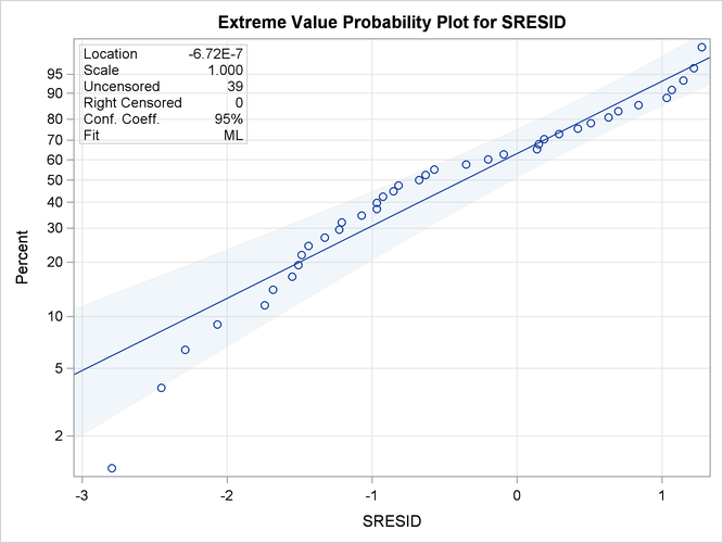
Although the estimated location is near zero and the estimated scale is near one, the plot reveals systematic curvature, indicating that the Weibull regression model might be inadequate.