Preliminary Analysis :: SAS/QC(R) 12.1 User's Guide

Preliminary Analysis

The following statements use the MVPMODEL procedure to conduct a preliminary principal component analysis:

ods graphics on;
proc mvpmodel data=MWflightDelays;
   var AA CO DL F9 FL NW UA US WN; 
run;

The DATA= option specifies the input data set, which contains the process measurement variables. The VAR statement specifies the process measurement variables to be analyzed. The ODS GRAPHICS ON statement enables ODS Graphics, which is used to produce plots for interpreting the model.

The procedure first outputs a summary of the model and the data, as shown in Figure 12.1.

Figure 12.1: Summary of Model and Data Information

The MVPMODEL Procedure

Data Set	WORK.MWFLIGHTDELAYS
Number of Variables	9
Missing Value Handling	Exclude
Number of Observations Read	16
Number of Observations Used	16
Number of Principal Components	9

This output includes the number of principal components in the model and the number of variables. In this case the procedure produces a model with nine principal components by default, because there are nine process variables.

Next, the procedure outputs the correlation matrix shown in Figure 12.2.

Figure 12.2: Correlation Matrix

Correlation Matrix
	AA	CO	DL	F9	FL	NW	UA	US	WN
AA	1.0000	0.5640	0.5206	0.4874	0.5403	0.4860	0.6466	0.7856	0.5506
CO	0.5640	1.0000	0.7855	0.6580	0.8519	0.6421	0.7672	0.8415	0.6526
DL	0.5206	0.7855	1.0000	0.8231	0.7598	0.4782	0.4951	0.7463	0.4525
F9	0.4874	0.6580	0.8231	1.0000	0.5119	0.2279	0.3509	0.6832	0.3914
FL	0.5403	0.8519	0.7598	0.5119	1.0000	0.6807	0.6975	0.8207	0.7186
NW	0.4860	0.6421	0.4782	0.2279	0.6807	1.0000	0.6715	0.5598	0.3970
UA	0.6466	0.7672	0.4951	0.3509	0.6975	0.6715	1.0000	0.7540	0.7736
US	0.7856	0.8415	0.7463	0.6832	0.8207	0.5598	0.7540	1.0000	0.8152
WN	0.5506	0.6526	0.4525	0.3914	0.7186	0.3970	0.7736	0.8152	1.0000

There are strong correlations (greater than 0.8) between variable pairs F9 and DL, CO and FL, and US and WN. This is not surprising, because these pairs of airlines have closely located hubs or focus cities.

The procedure also outputs the eigenvalue and variance information shown in Figure 12.3.

Figure 12.3: Eigenvalue and Variance Information

Eigenvalues of the Correlation Matrix
	Eigenvalue	Difference	Proportion	Cumulative
1	6.09006397	5.02872938	0.6767	0.6767
2	1.06133459	0.36642409	0.1179	0.7946
3	0.69491050	0.16102099	0.0772	0.8718
4	0.53388951	0.28357563	0.0593	0.9311
5	0.25031387	0.09537517	0.0278	0.9589
6	0.15493870	0.03339131	0.0172	0.9762
7	0.12154739	0.06166364	0.0135	0.9897
8	0.05988375	0.02676604	0.0067	0.9963
9	0.03311771		0.0037	1.0000

The eigenvalues are the variances of the principal components, and the proportions reflect the relative amount of variance explained by each component. The eigenvalues and the proportions are ordered from largest to smallest. Recall that principal components are orthogonal linear combinations of the variables that maximize variance in orthogonal directions.

More than 85% of the variance is explained by the first three principal components, as shown in the cumulative variance column. This suggests that a model with three principal components is adequate; this is confirmed by the plots in Figure 12.4.

Figure 12.4 shows a paneled display, with a scree plot in the left panel and a variance-explained plot in the right panel.

Figure 12.4: Scree Plot and Variance-Explained Plot

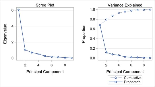
The scree plot shows the eigenvalues for each principal component. Traditionally, the scree plot has been recommended as an aid in selecting the number of principal components for the model by examining the “knee” in the plot (Mardia, Kent, and Bibby, 1979). The variance-explained plot shows both the proportion of variance and the cumulative variance explained by the principal components.