Example 12.1 Using Cross Validation to Select the Number of Principal Components

This example uses cross validation to select the number of principal components in a model. It uses the chromatography data from McReynolds (1970), which is also used in Wold (1978) and Eastment and Krzanowski (1982). The following statements create the chromatography data set:

data mcreynolds;
   input x1 - x10;
   datalines; 
 653    590    627    652    699    690    818    841    654    1006
 654    591    628    654    701    691    818    842    655    1006
 665    592    624    653    710    690    828    843    659    1014
 662    595    629    658    710    692    827    843    660    1012
 663    595    630    659    712    693    829    843    663    1013
 664    596    629    659    712    692    830    843    663    1015
 667    604    635    669    720    700    833    846    668    1016
 684    612    642    682    739    702    850    851    682    1035
 685    612    642    684    741    703    853    852    685    1039

   ... more lines ...   

1247   1447   1386   1683   1616   1370   1327   1220   1508    1275
1300   1509   1424   1695   1675   1403   1362   1229   1571    1305
1343   1581   1480   1762   1699   1463   1375   1212   1618    1285
;

The observations are liquid phases, and the variables are compounds. The value is the retention index for liquid phase in compound . The retention index values in the original article had the value of squalane subtracted from them. In this data set, the values have been corrected by adding the retention indices for squalane to all observations.

The following statements use the MVPMODEL procedure to select the number of principal components by using one-at-a-time cross validation:

proc mvpmodel data=mcreynolds plots=(scree cvplot) noscale cv=one;
run;

The CV= option specifies which method of cross validation to use to produce model diagnostics; in this case one-at-a-time cross validation is used. The PLOTS= option produces only the combination scree plot and variance-explained plot in addition to the cross validation plots.

Output 12.1.1 shows the model and data set information.

Output 12.1.1: Summary of Model and Data Set Information

The MVPMODEL Procedure

Data Set	WORK.MCREYNOLDS
Number of Variables	10
Missing Value Handling	Exclude
Number of Observations Read	226
Number of Observations Used	225
Maximum Number of Principal Components	9
Validation Method	Leave-one-out Cross Validation

Output 12.1.1 shows that one observation, liquid phase 69 (Triton X-400), was omitted because of a missing value. Also, notice that the maximum number of principal components is $\min \left( 15, nvar, nobs \right)-1=9$ , which is less than the number of variables; this is described in detail in Eastment and Krzanowski (1982).

The root mean PRESS values and the W statistic are shown in Output 12.1.2.

Output 12.1.2: Residual Summary

Cross Validation for the Number of Components
Number of Components	Root Mean PRESS	W
0	974.3136	.
1	30.77631	9586.179
2	26.85973	2.707278
3	26.49878	0.211824
4	22.94873	2.261922
5	21.50501	0.810642
6	20.91568	0.279385
7	20.53967	0.14514
8	20.25766	0.082967
9	20.03932	0.04342

In this case the index of the last W statistics greater than one is , suggesting a model with four components as shown in Output 12.1.3.

Output 12.1.3: Cross Validation Results

Number of Components Suggested by W Statistic	4

You can also use scree and variance-explained plots to select the number of principal components, as shown in Output 12.1.4.

Output 12.1.4: Scree and Variance-Explained Plots

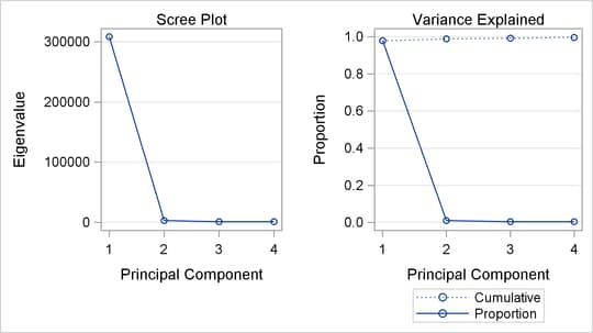
The plots in Output 12.1.4 indicate that one or two principal components explain almost all the variation.

The W statistic and plots are shown in Output 12.1.5.

Output 12.1.5: Cross Validation Analysis

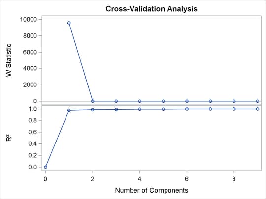
The cross validation plot is produced only when you specify both the CV= option and PLOTS=ALL or PLOTS=CVPLOT.

It is interesting that the cross validation methods of Wold (1978) and Eastment and Krzanowski (1982) choose five and four components, respectively, for this model, whereas a visual examination of the knee in the scree plot might suggest using only one or two components.