Getting Started: MVPMODEL Procedure

This example illustrates the basic features of the MVPMODEL procedure using airline flight delay data available from the U.S. Bureau of Transportation Statistics at http://www.transtats.bts.gov. The example applies multivariate process monitoring to flight delays.

Suppose you want to use a principal components model to create and SPE charts to monitor the variation in flight delays. These charts are appropriate because the data are multivariate and correlated.

The following statements create a SAS data set named MWflightDelays which provides the delays for flights that originate in the Midwestern U.S. The data set contains variables for nine airlines: AA (American Airlines), CO (Continental Airlines), DL (Delta Airlines), F9 (Frontier Airlines), FL (AirTran Airways), NW (Northwest Airlines), UA (United Airlines), US (US Airways), and WN (Southwest Airlines).

data MWflightDelays;
   format flightDate MMDDYY8.;
   label flightDate='Date';
   input flightDate :MMDDYY8. AA CO DL F9 FL NW UA US WN; 
   datalines; 
02/01/07 14.9  7.1  7.9  8.5 14.8  4.5  5.1 13.4  5.1
02/02/07 14.3  9.6 14.1  6.2 12.8  6.0  3.9 15.3 11.4
02/03/07 23.0  6.1  1.7  0.9 11.9 15.2  9.5 18.4  7.6
02/04/07  6.5  6.3  3.9 -0.2  8.4 18.8  6.2  8.8  8.0
02/05/07 12.0 14.1  3.3 -1.3 10.0 13.1 22.8 16.5 11.5

   ... more lines ...   

02/16/07 31.2 20.8 15.2 20.1  9.1 12.9 22.9 36.4 16.4
; 

The observations for a given date are the average flight delays in minutes for flights that depart from the Midwestern U.S. For example, on February 2, 2007, F9 (Frontier Airlines) departed 6.2 minutes late on average.

Preliminary Analysis

The following statements use the MVPMODEL procedure to carry out a preliminary principal components analysis:

ods graphics on;
proc mvpmodel data=MWflightDelays;
   var AA CO DL F9 FL NW UA US WN; 
run;

The DATA= option specifies the input data set, which contains the process measurement variables. The VAR statement specifies the process measurement variables to be analyzed. The ODS GRAPHICS ON statement enables ODS Graphics, which is used to produce plots for interpreting the model.

The procedure first outputs a summary of the model and the data, as shown in Figure 10.1.

Figure 10.1 Summary of Model and Data Information

The MVPMODEL Procedure

Data Set	WORK.MWFLIGHTDELAYS
Number of Variables	9
Missing Value Handling	Exclude
Number of Observations Read	16
Number of Observations Used	16
Number of Principal Components	9

This output includes the number of principal components in the model and the number of variables. By default, the procedure produces a model with nine principal components for this example.

Next the procedure outputs the correlation matrix shown in Figure 10.2.

Figure 10.2 Correlation Matrix

Correlation Matrix
	AA	CO	DL	F9	FL	NW	UA	US	WN
AA	1.0000	0.5640	0.5206	0.4874	0.5403	0.4860	0.6466	0.7856	0.5506
CO	0.5640	1.0000	0.7855	0.6580	0.8519	0.6421	0.7672	0.8415	0.6526
DL	0.5206	0.7855	1.0000	0.8231	0.7598	0.4782	0.4951	0.7463	0.4525
F9	0.4874	0.6580	0.8231	1.0000	0.5119	0.2279	0.3509	0.6832	0.3914
FL	0.5403	0.8519	0.7598	0.5119	1.0000	0.6807	0.6975	0.8207	0.7186
NW	0.4860	0.6421	0.4782	0.2279	0.6807	1.0000	0.6715	0.5598	0.3970
UA	0.6466	0.7672	0.4951	0.3509	0.6975	0.6715	1.0000	0.7540	0.7736
US	0.7856	0.8415	0.7463	0.6832	0.8207	0.5598	0.7540	1.0000	0.8152
WN	0.5506	0.6526	0.4525	0.3914	0.7186	0.3970	0.7736	0.8152	1.0000

There are strong correlations (greater than ) between variables F9 and DL, CO and FL, and US and WN. This is not surprising since these pairs have closely located hubs or focus cities.

The procedure also outputs eigenvalues and variance information shown in Figure 10.3.

Figure 10.3 Eigenvalue and Variance Information

Eigenvalues of the Correlation Matrix
	Eigenvalue	Difference	Proportion	Cumulative
1	6.09006397	5.02872938	0.6767	0.6767
2	1.06133459	0.36642409	0.1179	0.7946
3	0.69491050	0.16102099	0.0772	0.8718
4	0.53388951	0.28357563	0.0593	0.9311
5	0.25031387	0.09537517	0.0278	0.9589
6	0.15493870	0.03339131	0.0172	0.9762
7	0.12154739	0.06166364	0.0135	0.9897
8	0.05988375	0.02676604	0.0067	0.9963
9	0.03311771		0.0037	1.0000

The eigenvalues are the variances of the principal components, and the proportions reflect the relative amount of variance explained by each component. The eigenvalues and the proportions are ordered from largest to smallest. Recall that principal components are orthogonal linear combinations of the variables that maximize variance in orthogonal directions.

More than of the variance is explained by the first three principal components, as shown in the cumulative variance column. This suggests that a model with three principal components is adequate, and is confirmed by the plots in Figure 10.4.

Figure 10.4 shows a paneled display, with a scree plot in the first panel and a variance-explained plot in the second panel.

Figure 10.4 Scree Plot and Variance-Explained Plot

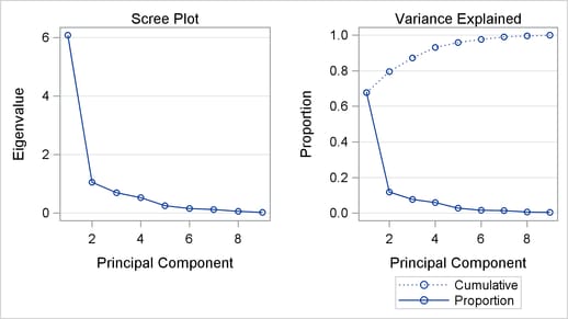
The scree plot shows the eigenvalues for each principal component. Traditionally, this plot has been recommended as an aid in selecting the number of principal components for the model by examining the "knee" in the plot (Mardia, Kent, and Bibby; 1979). The variance-explained plot shows both the proportion of variance and cumulative variance explained by the principal components.

Building a Principal Components Model

To build a model with only three principal components, you can use the NCOMP= option as shown in the following statements:

proc mvpmodel data=MWflightDelays ncomp=3 plots=all out=outDelays;
   var AA CO DL F9 FL NW UA US WN; 
run;

The PLOTS=ALL option requests all possible plots, which include pairwise plots of the principal components scores and loadings in addition to the default scree plot and variance-explained plot. The OUT= option produces an output data set with principal component scores, statistics, residuals, SPE statistics, and more as described in the section Output Data Sets. Note that ODS Graphics is still enabled, so you do not need to specify the ODS GRAPHICS ON statement here.

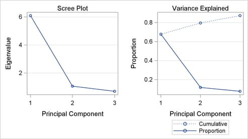
The correlation matrix is the same as in Figure 10.2. The eigenvalue information, scree plot, and variance-explained plot are similar to Figure 10.3 and Figure 10.4. However, the use of the NCOMP=3 option results in outputs that show information only for the three components in the model, seen in Figure 10.5 and Figure 10.6.

Figure 10.5 Eigenvalue and Variance Information

The MVPMODEL Procedure

Eigenvalues of the Correlation Matrix
	Eigenvalue	Difference	Proportion	Cumulative
1	6.09006397	5.02872938	0.6767	0.6767
2	1.06133459	0.36642409	0.1179	0.7946
3	0.69491050		0.0772	0.8718

Figure 10.6 Scree Plot and Variance-Explained Plot

Also, the model summary, shown in Figure 10.7, is different since there are now only three principal components in the model.

Figure 10.7 Summary of Model and Data Information

The MVPMODEL Procedure

Data Set	WORK.MWFLIGHTDELAYS
Number of Variables	9
Missing Value Handling	Exclude
Number of Observations Read	16
Number of Observations Used	16
Number of Principal Components	3

The OUT= data set partially listed in Figure 10.8 contains and SPE statistics based on the model with three principal components, in addition to the original variables and other observationwise statistics.

Figure 10.8 Partial Listing of Output Data Set outDelays

flightDate	AA	CO	DL	F9	FL	NW	UA	US	WN	Prin1	Prin2	Prin3	_NOBS_	_TSQUARE_	R_AA	R_CO	R_DL	R_F9	R_FL	R_NW	R_UA	R_US	R_WN	_SPE_
02/01/07	14.9	7.1	7.9	8.5	14.8	4.5	5.1	13.4	5.1	-1.08708	1.20953	-0.03839	16	1.57457	-0.05779	-0.18178	-0.01835	-0.15280	0.87457	-0.37864	-0.06037	-0.12896	-0.02300	0.98911
02/02/07	14.3	9.6	14.1	6.2	12.8	6.0	3.9	15.3	11.4	-0.65786	1.26249	0.11447	16	1.59169	-0.17802	-0.16663	0.68047	-0.62682	0.49289	-0.35101	-0.27027	-0.14161	0.41169	1.54414
02/03/07	23.0	6.1	1.7	0.9	11.9	15.2	9.5	18.4	7.6	-0.86457	-0.73183	0.29270	16	0.75065	0.54274	-0.30297	-0.20552	-0.02408	0.31360	0.21270	-0.49772	0.24287	-0.23829	0.93626
02/04/07	6.5	6.3	3.9	-0.2	8.4	18.8	6.2	8.8	8.0	-1.50578	-0.69718	1.32511	16	3.35709	-0.25729	-0.24974	0.05624	0.05279	-0.02427	0.29305	-0.44076	0.13493	0.50899	0.69253
02/05/07	12.0	14.1	3.3	-1.3	10.0	13.1	22.8	16.5	11.5	-0.63903	-1.11141	0.38617	16	1.44549	-0.44128	0.28274	0.09998	-0.15050	0.00176	-0.36866	0.39124	0.07233	-0.06265	0.60545

The variables Prin1, Prin2, and Prin3 contain the principal component scores. Variables R_AA through R_WN are the residuals for each of the original variables. The contents of the OUT= data set are described in the section Output Data Sets. See the section Principal Components Analysis for computational details of the results saved in the output data set.

The PLOTS=ALL option produces score plots for pairs of principal components in the model. Two of these plots are shown in Figure 10.9 and Figure 10.10:

Figure 10.9 Score Plot for Principal Components One and Two

Figure 10.10 Score Plot for Principal Components One and Three

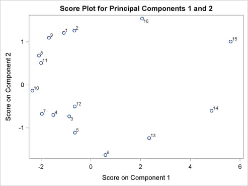
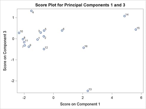
A score plot is simply a scatter plot of the scores for two principal components. The labels indicate the observation numbers of the points. By examining clusters and outliers in these plots, you can better understand the relationships among the observations and the variation in the process. For example, the points labeled 13 through 16 are extreme points in the direction of the first principal component. The directions of the principal components are not uniquely determined, so external information is needed to interpret which direction indicates behind or ahead of schedule. These points represent flight delays between February 13, 2007, and February 16, 2007, when there was a major winter storm.

Figure 10.11 displays one of the three loading plots that are produced. A loading plot is a scatter plot of the variable loadings for a pair of principal components, and it helps you understand the relationships among the variables.

Figure 10.11 Loading Plot for Principal Components One and Two

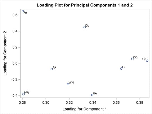
Loadings are the variable coefficients in the eigenvectors (linear combination of variables) that defines the principal component. The loadings explain how variables contribute to the linear combination. Here, the loadings for the first principal component are all positive and are all similar in value, which suggests that the first principal component describes the average delay. The second principal component appears to be a contrast between the delays for F9, DL, CO, and US and the remaining airlines. See the section Principal Components Analysis for more information about the details and interpretation of principal components loadings and scores.

The OUT= data set is used as an input to the MVPMONITOR procedure, described in Chapter 11, The MVPMONITOR Procedure. The MVPMONITOR procedure creates charts for the and SPE statistics, and the charts for this example are created in Example 10.2 and in the MVPMONITOR procedure.