Example 10.2 Creating a Classical T-Square Chart
Using the MVPMODEL procedure to create a classical  chart is straightforward.
proc mvpmodel data=flightDelays(where=(region='NE')) ncomp=9
              plots=none out=mvpout timegroup=flightDate;
   var AA CO DL F9 FL NW UA US WN;
run;
Simply use the NCOMP= option to set the number of principal components used in the model to equal the number of variables in the model. There are nine variables in the VAR statement, so setting NCOMP=9 creates an output data set for a classical chart. The MVPMONITOR procedure creates the classical chart.
proc mvpmonitor history=mvpout;
   time flightDate;
   tsquarechart;
run;
The mvpout data set produced by the MVPMODEL procedure contains the classical statistic for each observation. In this data set there are six observations per time point—one for each region. The WHERE statement in the MVPMONITOR procedure selects the region to be charted, and the TSQUARECHART statement specifies a chart output. The classical chart is shown in Output 10.2.1.
Chart
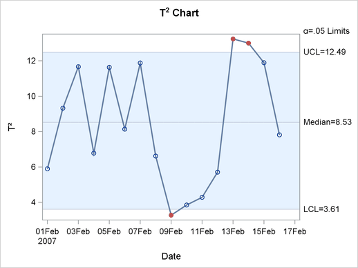
In this case, the classical chart finds out-of-control observations above the upper control limit during February 14-16, and below the lower control limit on February 1, 10, and 12.
The OUT= data set shown in Output 10.2.2 contains statistics based on the model with nine principal components, in addition to the original variables and other observationwise statistics.
| flightDate | region | AA | CO | DL | F9 | FL | NW | UA | US | WN | Prin1 | Prin2 | Prin3 | Prin4 | Prin5 | Prin6 | Prin7 | Prin8 | Prin9 | _NOBS_ | _TSQUARE_ |
|---|---|---|---|---|---|---|---|---|---|---|---|---|---|---|---|---|---|---|---|---|---|
| 02/01/07 | NE | 15.7 | 7.1 | 8.6 | 6.3 | 14.6 | 6.2 | 7.0 | 11.0 | 6.4 | -1.21243 | 0.17834 | 0.22056 | -0.79000 | -0.48268 | 0.34300 | -0.02352 | -0.14347 | -0.10508 | 16 | 5.8964 |
| 02/02/07 | NE | 16.0 | 19.4 | 10.7 | 6.4 | 19.0 | 6.1 | 8.3 | 14.4 | 14.2 | -0.45475 | 0.16238 | 0.14289 | -1.04539 | -0.50018 | -0.17205 | 0.45608 | -0.13206 | 0.05144 | 16 | 9.3287 |
| 02/03/07 | NE | 14.5 | 1.5 | 5.4 | 13.3 | 13.6 | 9.7 | 16.6 | 7.5 | 9.9 | -1.02441 | 0.14289 | 0.17630 | -0.27007 | 0.18032 | 0.76339 | 0.04135 | 0.31670 | 0.13645 | 16 | 11.6631 |
| 02/04/07 | NE | 12.4 | 14.3 | 5.8 | 0.7 | 11.8 | 20.1 | 11.2 | 8.6 | 8.1 | -0.92324 | -0.50925 | 0.60010 | 0.23665 | -0.89035 | -0.24846 | 0.04209 | 0.19427 | 0.07218 | 16 | 6.7821 |
| 02/05/07 | NE | 19.8 | 27.6 | 7.3 | 16.1 | 13.3 | 14.8 | 39.9 | 16.4 | 9.7 | 0.52789 | 0.27352 | -0.71527 | 0.90787 | 0.22967 | 0.10383 | 0.53617 | -0.05627 | -0.13310 | 16 | 11.6280 |
No SPE statistics are produced when the number of principal components equals the number of process variables.
Note: This procedure is experimental.