The GANTT Procedure
- Overview
- Getting Started
-
Syntax

-
DetailsSchedule Data SetMissing Values in Input Data SetsSpecifying the PADDING= OptionPage FormatMultiple Calendars and HolidaysFull-Screen VersionGraphics VersionSpecifying the Logic OptionsAutomatic Text AnnotationWeb-Enabled Gantt ChartsMode-Specific DifferencesDisplayed OutputMacro Variable _ORGANTTComputer Resource RequirementsODS Style Templates
-
ExamplesLine-Printer ExamplesPrinting a Gantt ChartCustomizing the Gantt ChartGraphics ExamplesMarking HolidaysMarking Milestones and Special DatesUsing the COMPRESS OptionUsing the MININTERVAL= and SCALE= OptionsUsing the MINDATE= and MAXDATE= OptionsVariable-Length HolidaysMultiple CalendarsPlotting the Actual ScheduleComparing Progress Against a Baseline ScheduleUsing the COMBINE OptionPlotting the Resource-Constrained ScheduleSpecifying the Schedule Data DirectlyBY ProcessingGantt Charts by PersonsUsing the HEIGHT= and HTOFF= OptionsDrawing a Logic Gantt Chart Using AON RepresentationSpecifying the Logic Control OptionsNonstandard Precedence RelationshipsUsing the SAS/GRAPH ANNOTATE= OptionUsing the Automatic Text Annotation FeatureMultiproject Gantt ChartsMultisegment Gantt ChartsZoned Gantt ChartsWeb-Enabled Gantt ChartsUsing the CHARTWIDTH= OptionUsing the TIMEAXISFORMAT= OptionStatement and Option Cross-Reference Tables
- References
Specifying the Logic Options
The Logic options are a family of options used with the GANTT procedure that enable you to view the precedence relationships between activities on the Gantt chart. The Logic options constitute a high-resolution graphics feature and, as such, are only valid with specification of the GRAPHICS option in the PROC GANTT statement. The Logic options can accommodate nonstandard precedence relationships. The Logic options enable you to control the color, line style, and width of the connecting arcs as well as their layout and positioning on the Gantt chart. You can specify the precedence information required to draw the connections in one of two formats and store it in a data set different from the Schedule data set. You can also use the Schedule data set produced by PROC CPM to provide the precedence information. When using the Schedule data set from PROC CPM , you can ensure that all the relevant precedence information exists in the data set by either specifying the XFERVARS option in the PROC CPM statement or by using an ID statement.
The Logic options are not valid with the specification of either a BY statement or the COMBINE option in the CHART statement.
In order to invoke the logic options, you need to, minimally, specify a set of variables that defines the precedence relationships between tasks. This can be done using one of two formats for defining project networks, the AOA specification or the AON specification.
Activity-on-Arc (AOA) Specification
In the AOA specification, each activity of the project is represented by an arc. The node at the tail of the arc represents the start of the activity, and the node at the head of the arc represents the finish of the activity. The relationship between an activity and its successor is represented by setting the tail node of the successor arc to be the head node of the activity arc. One of the disadvantages of using the AOA method is that it cannot accommodate nonstandard lag types; all lag types are of the Finish-to-Start (FS) type.
The variables required by PROC GANTT to establish a valid AOA specification are defined using the HEADNODE= and TAILNODE= options in the CHART statement.
Activity-on-Node (AON) Specification
In the AON specification, each activity is represented by a node. All arcs originating from an activity terminate at its successors. Consequently, all arcs terminating at an activity originate from its predecessors.
The variables required by PROC GANTT to establish a valid AON specification are defined by the ACTIVITY= and SUCCESSOR= options in the CHART statement.
Optionally, nonstandard precedence relationships can be specified using the LAG= option in the CHART statement to define a variable that defines the lag type of a relationship.
Precedence Data Set
When using the AON specification, you can specify the precedence information using a data set different from the Schedule data set. This is particularly useful when producing several Gantt charts for the same project with different schedule information as would typically be the case when monitoring a project in progress. It eliminates the requirement that the precedence information exist in each Schedule data set and enables for more compact data. This separate data set is specified by the PRECDATA= option in the PROC GANTT statement statement and is referred to as the Precedence data set.
In order to graphically represent the precedence relationships derived from the Precedence data set on the Gantt chart, you must link the Precedence data set with the Schedule data set by means of a common variable. This common variable is selected as the ACTIVITY variable by virtue of the fact that it always exists in the Precedence data set. Thus, when using the Precedence data set, you need to ensure that the ACTIVITY variable exists in the Schedule data set, too.
In the event that both a valid AOA and a valid AON specification exist, PROC GANTT uses the AON specification by default. To override the default, use the AOA option in the CHART statement.
Drawing the Precedence Connections
The relationship between an activity and its successor is represented on the Gantt chart by a series of horizontal and vertical line segments that connect their schedule bars corresponding to a specified type (early/late, actual, and so forth). For a given connection, the intersection of a horizontal segment with a vertical segment is called a turning point of the connection. The type of the schedule bar used for the connection, also called the logic bar, is determined by the LEVEL= option in the CHART statement.
Every connection is comprised of either three or five segments and is termed a 3-segment or a 5-segment connection, respectively. The segments are routed in the following sequence:
-
a horizontal segment that originates from the appropriate end of the logic bar corresponding to the activity. The length of this segment is controlled by the MINOFFGV= and MININTGV= options in the CHART statement.
-
a vertical segment traveling from activity to the successor
-
a horizontal segment traveling towards the appropriate end of the successor’s logic bar. The length of this segment is determined by the MINOFFLV= and MAXDISLV= options in the CHART statement.
-
a vertical and horizontal segment into the logic bar of the successor
Every connection begins with a horizontal line segment originating from the activity’s logic bar and ends with a a horizontal line segment terminating at the successor’s logic bar. If the lag type of the relationship is SS or SF, the initial horizontal segment originates from the left end of the activity’s logic bar, otherwise it originates from the right end of the logic bar. If the lag type of the relationship is SS or FS, the final horizontal segment terminates at the left end of the successor’s logic bar, otherwise it terminates at the right end of the logic bar.
Note: The ends of the bars must be consistent with the lag type of the connection if it is to be drawn; that is, the left end of the activity’s logic bar must represent a start time if an SS or SF lag type connection is to be drawn, and the right end of the activity’s logic bar must represent a finish time if an FS or FF lag type connection is to be drawn.
Violation of these conditions is unlikely when using the Schedule data set generated by PROC CPM
. An example violating these conditions is a Schedule data set containing incorrect or invalid data. The following example
illustrates two observations that are in violation of these conditions. The first observation is invalid data (E_START greater than E_FINISH) while the second observation is incomplete (missing E_START and L_FINISH times).
             E_START   E_FINISH  L_START  L_FINISH
             03MAR04   01MAR04      .         .
                .      05MAR04   07MAR04      .
The following figure illustrates two typical precedence connections between an activity and its successor.
                  ACTIVITY  SUCCESSOR   LAG
                     A          C       FS
                     B          C       FS
Figure 8.10: Typical Precedence Connections
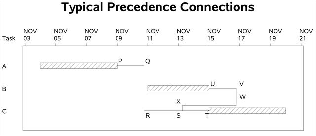
The connection from activity A to activity C is comprised of three segments PQ, QR, and RT whereas the connection from activity B to activity C is made up of five segments UV, VW, WX, XS, and ST; the two additional segments correspond to the optional segments mentioned in item d) above. Points Q, R, V, W, X, and S are turning points.
Formatting the Axis
If neither MINDATE= nor MAXDATE= have been specified, the time axis of the Gantt chart is extended by a small amount in the appropriate direction or directions in an attempt to capture all of the relevant precedence connections on the chart. While this will succeed for the majority of Gantt charts, it is by no means guaranteed. If connection lines still tend to run off the chart, you can perform one or both of the following tasks.
-
Use the MINDATE= or MAXDATE= options (or both) in the CHART statement to increase the chart range as necessary.
-
Decrease the values of the MINOFFGV= , MININTGV= , MAXDISLV= , and MINOFFLV= options to reduce the horizontal range spanned by the vertical segments so that they will lie within the range of the time axis.
On the other hand, if the automatic extension supplied by PROC GANTT is excessive, you can suppress it by specifying the NOEXTRANGE option in the CHART statement.
The following section, "Controlling the Layout," addresses the CHART statement options MINOFFGV=, MININTGV=, MINOFFLV=, and MAXDISLV= which control placement of the vertical segments that make up a connection. For most Gantt charts, default values of these options will suffice since their usage is typically reserved for "fine tuning" chart appearance. This section can be skipped unless you want to control the layout of the connection. The description of the layout methodology and concepts is also useful to help you understand the routing of the connections in a complex network with several connections of different types.
Controlling the Layout
The concepts of global and local verticals are first introduced in order to describe the function of the segment placement controls.
Global Verticals
In the interest of minimizing clutter on the chart, each activity is assigned a maximum of two vertical tracks for placement of the vertical segment described in item b) above. One vertical track is maintained for SS and SF lag type connections and is referred to as the start global vertical of the activity, while the other vertical track is maintained for FS and FF lag type connections and is referred to as the finish global vertical of the activity. The term global vertical refers to either start global vertical or finish global vertical.
Note: The use of the term "global" is attributed to the fact that in any connection from an activity to its successor, the global vertical of the activity corresponds to the only segment that travels from activity to successor.
Figure 8.11 illustrates the two global verticals of activity A.
Figure 8.11: Global Verticals
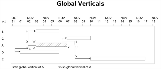
Activity A has four successors: activities B, C, D, and E. The lag type of the relationship between A and B is nonstandard, namely 'Start-to-Start', as is that between A and D. The other two lag types are standard. The start and finish global verticals of activity A are represented by the two dotted lines. The vertical segments of the SS lag type connections from A to B and from A to D that are placed along the start global vertical of A are labeled PQ and RS, respectively. The vertical segments of the FS lag type connections from A to C and from A to E that are placed along the finish global vertical of A are labeled TU and UV, respectively.
For a given connection from activity to successor, the vertical segment that is placed on the activity global vertical is connected to the appropriate end of the logic bar by the horizontal segment described in item a) above. The minimum length of this horizontal segment is specified with the MINOFFGV= option in the CHART statement. Further, the length of this segment is affected by the MININTGV= option in the CHART statement, which is the minimum interdistance of any two global verticals. In Figure 8.11, the horizontal segments QW and RX connect the vertical segments PQ and RS, respectively, to the logic bar and the horizontal segment YU connects both vertical segments TU and UV to the logic bar.
Local Verticals
Each activity has seven horizontal tracks associated with it, strategically positioned on either end of the logic bar, above the first bar of the activity, and below the last bar of the activity. These tracks are used for the placement of the horizontal segments described in items c) and d), respectively.
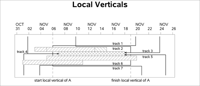
Figure 8.12 illustrates the positions of the horizontal tracks for an activity in a Gantt chart with four schedule bars. Three of the horizontal tracks, namely track 1, track 4, and track 7, service the start of the logic bar and are connected to one another by a vertical track referred to as the Start Local Vertical. Similarly, the horizontal tracks track 2, track 3, track 5, and track 6 service the finish of the bar and are interconnected by a vertical track referred to as the Finish Local Vertical. The local verticals are used for placement of the vertical segment described in item d) above.
Note: The use of the term "local" is attributed to the fact that the local vertical is used to connect horizontal tracks associated with the same activity.
Notice that track 1 and track 7 terminate upon their intersection with the start local vertical and that track 2 and track 6 terminate upon their intersection with the finish local vertical.
The minimum distance of a local vertical from its respective bar end is specified with the MINOFFLV= option in the CHART statement. The maximum displacement of the local vertical from this point is specified using the MAXDISLV= option in the CHART statement. The MAXDISLV= option is used to offset the local vertical in order to prevent overlap with any global verticals.
Arrowheads are drawn by default on the horizontal tracks corresponding to the logic bar, namely track 3, track 4, and track 5, upon entering the bar and on continuing pages. The NOARROWHEAD option is used to suppress the display of arrowheads.
Figure 8.12: Local Verticals
Routing the Connection
The routing of the precedence connection from an activity to its successor is dependent on two factors, namely
-
the horizontal displacement of the appropriate global vertical of the activity relative to the appropriate local vertical of the successor
-
the vertical position on the task axis of the activity relative to the successor
The routing of a SS or FS type precedence connection from activity to successor is described below. A similar discussion holds for the routing of a SF or FF type precedence connection.
Suppose the activity lies above the successor. Let the start local vertical of the successor be denoted by slv, and let the appropriate global vertical of the activity be denoted by gv.
Case 1:
If gv lies to the left of slv, then the connection is routed vertically down along gv onto track 4 of the successor, on which it is routed horizontally to enter the bar. The resulting 3-segment connection is shown in Figure 8.13.
Figure 8.13: 3-Segment Connection
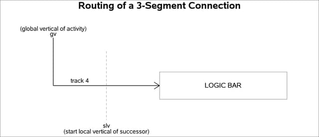
An example of this type of routing is illustrated by the connection between activities A and C in Figure 8.10.
Case 2:
If gv lies to the right of slv, then the connection is routed vertically down along gv onto track 1 of the successor, horizontally to the left to meet slv, vertically down along slv onto track 4 of the successor and horizontally to the right to enter the bar. The resulting 5-segment connection is shown in Figure 8.14.
Figure 8.14: 5-Segment Connection
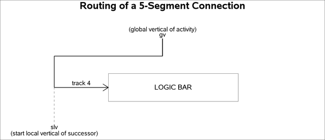
This type of routing is illustrated by the connection between activities B and C in Figure 8.10.
An identical description applies when the activity lies below the successor, with the only difference being that track 7 is used in place of track 1 (see Figure 8.12).