The Earned Value Management Macros

Consider the following set of activities that constitute a software multiproject. The Project variable defines the project hierarchy and the Succesr1 and Succesr2 variables define the precedence relationships. The complete project data is shown in Figure 11.6.
data softin;
   input Project  $10.
         Activity $11.
         Description $22.
         Duration
         Succesr1 $9.
         Succesr2 $9.;
   datalines;
          SWPROJ     Software project       .
DEBUG     RECODE     Recoding               5  DOCEDREV  QATEST
DOC       DOCEDREV   Doc. Edit and Revise  10  PROD
DOC       PRELDOC    Prel. Documentation   15  DOCEDREV  QATEST
MISC      MEETMKT    Meet Marketing         0  RECODE
MISC      PROD       Production             1
SWPROJ    DEBUG      Debug & Code Fixes     .
SWPROJ    DOC        Doc. Subproject        .
SWPROJ    MISC       Miscellaneous          .
SWPROJ    TEST       Test Subproject        .
TEST      QATEST     QA Test Approve       10  PROD
TEST      TESTING    Initial Testing       20  RECODE
;
Figure 11.6: Software Schedule Input SOFTIN
| Software Schedule Input |
| Obs | Project | Activity | Description | Duration | Succesr1 | Succesr2 |
|---|---|---|---|---|---|---|
| 1 | SWPROJ | Software project | . | |||
| 2 | DEBUG | RECODE | Recoding | 5 | DOCEDREV | QATEST |
| 3 | DOC | DOCEDREV | Doc. Edit and Revise | 10 | PROD | |
| 4 | DOC | PRELDOC | Prel. Documentation | 15 | DOCEDREV | QATEST |
| 5 | MISC | MEETMKT | Meet Marketing | 0 | RECODE | |
| 6 | MISC | PROD | Production | 1 | ||
| 7 | SWPROJ | DEBUG | Debug & Code Fixes | . | ||
| 8 | SWPROJ | DOC | Doc. Subproject | . | ||
| 9 | SWPROJ | MISC | Miscellaneous | . | ||
| 10 | SWPROJ | TEST | Test Subproject | . | ||
| 11 | TEST | QATEST | QA Test Approve | 10 | PROD | |
| 12 | TEST | TESTING | Initial Testing | 20 | RECODE |
The project network diagram showing the precedence relationships can be generated with the following code, using the NETDRAW procedure (see Chapter 9 for additional information). The resulting diagram is shown in Figure 11.7. (Note that the first DATA step removes the root task to simplify the diagram.)
data softabridged;
   set softin;
   if activity ne 'SWPROJ' and project ne 'SWPROJ' then output;
run;
proc netdraw data=softabridged out=ndout graphics;
   actnet/act=activity
   id=(description)
   nodefid
   nolabel
   succ=(succesr1 succesr2)
   lwidth=2
   coutline=black
   ctext=black
   carcs=black
   cnodefill=ltgray
   zone=project
   zonespace
   htext=3 pcompress
   centerid;
run;

The project hierarchy, or Work Breakdown Structure (WBS), can be visualized with the following code. The graphical output is shown in Figure 11.8. The details for the use of the %EVG_WBS_CHART macro are given in the section Syntax: Earned Value Management Macros.
%evg_wbs_chart(
   structure=softin,
   activity=activity,
   project=project
);

The CPM procedure can be used as follows to generate a schedule based on the precedence and hierarchical constraints (see Chapter 4 for more details).
proc cpm data=softin
         out=software
         interval=day
         date='01mar10'd;
   id description;
   project project / addwbs;
   activity activity;
   duration duration;
   successor succesr1 succesr2;
run;
The resulting schedule data set is manipulated to produce a data set containing the early and late schedules, shown in Figure 11.9.
The WBS_CODE variable gives the project hierarchy. The E_START and E_FINISH variables represent the early schedule, and the L_START and L_FINISH variables give the late schedule.
proc sort data=software;
   by wbs_code;
run;

proc print data=software;
    title 'Planned Schedule';
    var activity wbs_code e_start e_finish l_start l_finish;
run;
Figure 11.9: Software Schedule SOFTWARE
| Planned Schedule |
| Obs | Activity | WBS_CODE | E_START | E_FINISH | L_START | L_FINISH |
|---|---|---|---|---|---|---|
| 1 | SWPROJ | 0 | 01MAR10 | 05APR10 | 01MAR10 | 05APR10 |
| 2 | DEBUG | 0.0 | 21MAR10 | 25MAR10 | 21MAR10 | 25MAR10 |
| 3 | RECODE | 0.0.0 | 21MAR10 | 25MAR10 | 21MAR10 | 25MAR10 |
| 4 | DOC | 0.1 | 01MAR10 | 04APR10 | 11MAR10 | 04APR10 |
| 5 | DOCEDREV | 0.1.0 | 26MAR10 | 04APR10 | 26MAR10 | 04APR10 |
| 6 | PRELDOC | 0.1.1 | 01MAR10 | 15MAR10 | 11MAR10 | 25MAR10 |
| 7 | MISC | 0.2 | 01MAR10 | 05APR10 | 21MAR10 | 05APR10 |
| 8 | MEETMKT | 0.2.0 | 01MAR10 | 01MAR10 | 21MAR10 | 21MAR10 |
| 9 | PROD | 0.2.1 | 05APR10 | 05APR10 | 05APR10 | 05APR10 |
| 10 | TEST | 0.3 | 01MAR10 | 04APR10 | 01MAR10 | 04APR10 |
| 11 | QATEST | 0.3.0 | 26MAR10 | 04APR10 | 26MAR10 | 04APR10 |
| 12 | TESTING | 0.3.1 | 01MAR10 | 20MAR10 | 01MAR10 | 20MAR10 |
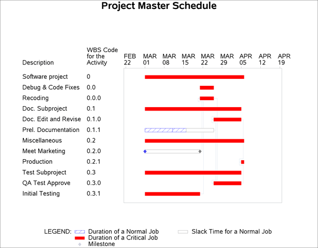
A Gantt chart of this schedule can be produced with the GANTT procedure using the following code. (See Chapter 8, for more details.)
goptions reset=symbol;
goptions reset=pattern;
pattern1 value=R1 color=B REPEAT=1;
pattern2 value=E color=GR REPEAT=1;
pattern3 value=S color=R REPEAT=1;
pattern4 value=X1 color=P REPEAT=1;
pattern5 value=E color=BR REPEAT=1;
pattern6 value=L1 color=GR REPEAT=1;
pattern7 value=R1 color=G REPEAT=1;
pattern8 value=X1 color=Y REPEAT=1;
pattern9 value=E color=B REPEAT=1;
title h=4pct 'Project Master Schedule';
title2 h=3pct;
proc gantt data=software;
   chart / mininterval=week pcompress
      height=1.3
      skip=2
      activity=activity
      nojobnum
      successor=(succesr1 succesr2)
      scale=10
      duration=duration;
      id description wbs_code;
run;
Figure 11.10 shows the output from this call to PROC GANTT.
Now suppose the early schedule is designated as the baseline. For the sake of clarity, the E_START and E_FINISH variables have been renamed to START and FINISH, respectively. Also, the variables required for performing the earned value analysis are retained. The modified data set
is shown in Figure 11.11.
data software;
   set software;
   keep project activity duration description
        e_start e_finish wbs_code succesr1 succesr2;
   rename e_start = Start
          e_finish = Finish;
   label wbs_code = 'WBS Code'
         e_start = 'Start'
         e_finish = 'Finish';
   if duration eq . then duration = proj_dur;
run;
Figure 11.11: Software Schedule SOFTWARE
| Planned Schedule |
| Obs | Activity | WBS Code | Description | Duration | Start | Finish |
|---|---|---|---|---|---|---|
| 1 | SWPROJ | 0 | Software project | 36 | 01MAR10 | 05APR10 |
| 2 | DEBUG | 0.0 | Debug & Code Fixes | 5 | 21MAR10 | 25MAR10 |
| 3 | RECODE | 0.0.0 | Recoding | 5 | 21MAR10 | 25MAR10 |
| 4 | DOC | 0.1 | Doc. Subproject | 35 | 01MAR10 | 04APR10 |
| 5 | DOCEDREV | 0.1.0 | Doc. Edit and Revise | 10 | 26MAR10 | 04APR10 |
| 6 | PRELDOC | 0.1.1 | Prel. Documentation | 15 | 01MAR10 | 15MAR10 |
| 7 | MISC | 0.2 | Miscellaneous | 36 | 01MAR10 | 05APR10 |
| 8 | MEETMKT | 0.2.0 | Meet Marketing | 0 | 01MAR10 | 01MAR10 |
| 9 | PROD | 0.2.1 | Production | 1 | 05APR10 | 05APR10 |
| 10 | TEST | 0.3 | Test Subproject | 35 | 01MAR10 | 04APR10 |
| 11 | QATEST | 0.3.0 | QA Test Approve | 10 | 26MAR10 | 04APR10 |
| 12 | TESTING | 0.3.1 | Initial Testing | 20 | 01MAR10 | 20MAR10 |
Assume also that each of the activities is budgeted to incur costs continuously at the rates shown in the RATES data set in Figure 11.12.
Figure 11.12: Software Budget RATES
| Planned Rates |
| Obs | Activity | Rate |
|---|---|---|
| 1 | SWPROJ | 5 |
| 2 | RECODE | 6 |
| 3 | PRELDOC | 4 |
| 4 | DOCEDREV | 4 |
| 5 | MEETMKT | . |
| 6 | PROD | 2 |
| 7 | TEST | 1 |
| 8 | DOC | 1 |
| 9 | MISC | 1 |
| 10 | DEBUG | 1 |
| 11 | TESTING | 3 |
| 12 | QATEST | 4 |
To determine the periodic budgeted costs, invoke the %EVA_PLANNED_VALUE macro as follows:
%eva_planned_value(
     plansched=software,      /* schedule data */
     activity=activity,
     start=start,
     finish=finish,
     duration=duration,
     budgetcost=rates,        /* cost data */
     rate=rate
);
The parameters used in this call to %EVA_PLANNED_VALUE are described in the following list. More details are given in the section Syntax: Earned Value Management Macros.
-
PLANSCHED= identifies the data set that contains the planned schedule.
-
ACTIVITY= specifies the activity variable in the PLANSCHED= and BUDGETCOST= data sets.
-
START= specifies the start date or datetime variable in the PLANSCHED= data set.
-
FINISH= specifies the finish date or datetime variable in the PLANSCHED= data set.
-
DURATION= specifies the task duration variable in the PLANSCHED= data set.
-
BUDGETCOST= identifies the data set containing the budgeted costs.
-
RATE= specifies the cost rate variable in the BUDGETCOST= data set.
The output data set generated by this call to %EVA_PLANNED_VALUE is shown in Figure 11.13.
Figure 11.13: Periodic Planned Value Data Set Using %EVA_PLANNED_VALUE
| Daily Planned Value |
| Obs | Date | PV Rate |
|---|---|---|
| 1 | 01MAR10 | 15 |
| 2 | 02MAR10 | 15 |
| 3 | 03MAR10 | 15 |
| 4 | 04MAR10 | 15 |
| 5 | 05MAR10 | 15 |
| 6 | 06MAR10 | 15 |
| 7 | 07MAR10 | 15 |
| 8 | 08MAR10 | 15 |
| 9 | 09MAR10 | 15 |
| 10 | 10MAR10 | 15 |
| 11 | 11MAR10 | 15 |
| 12 | 12MAR10 | 15 |
| 13 | 13MAR10 | 15 |
| 14 | 14MAR10 | 15 |
| 15 | 15MAR10 | 15 |
| 16 | 16MAR10 | 11 |
| 17 | 17MAR10 | 11 |
| 18 | 18MAR10 | 11 |
| 19 | 19MAR10 | 11 |
| 20 | 20MAR10 | 11 |
| 21 | 21MAR10 | 15 |
| 22 | 22MAR10 | 15 |
| 23 | 23MAR10 | 15 |
| 24 | 24MAR10 | 15 |
| 25 | 25MAR10 | 15 |
| 26 | 26MAR10 | 16 |
| 27 | 27MAR10 | 16 |
| 28 | 28MAR10 | 16 |
| 29 | 29MAR10 | 16 |
| 30 | 30MAR10 | 16 |
| 31 | 31MAR10 | 16 |
| 32 | 01APR10 | 16 |
| 33 | 02APR10 | 16 |
| 34 | 03APR10 | 16 |
| 35 | 04APR10 | 16 |
| 36 | 05APR10 | 8 |
Note that the “PV Rate” column shows the daily Planned Value (or Budgeted Cost of Work Scheduled). This is the cost incurred each day according to the plan or budget.
In general, once a project is in progress it is subject to uncertainties, the impact of which can often only be approximated in the original plan. Such uncertainties can affect the project schedule, project cost, or both. From a schedule standpoint an activity may be delayed due to a multitude of factors—a required resource being unavailable, a worker becoming sick, a machine breaking down, adverse weather conditions, etc. From a cost standpoint a contractor may revise his/her original estimate, the cost of raw materials may increase due to external factors, a sick or disabled worker might necessitate the use of a more costly contractor to minimize schedule slippage, etc.
Figure 11.14 lists the status of completed activities, and those in progress, as of March 25, 2010.
Figure 11.14: Software Project Status SOFTACT
| Actual Dates and Percentage Complete |
| Obs | Activity | Start | Finish | Percent |
|---|---|---|---|---|
| 1 | MEETMKT | 01MAR10 | 01MAR10 | 100 |
| 2 | PRELDOC | 01MAR10 | 14MAR10 | 100 |
| 3 | TESTING | 01MAR10 | . | 80 |
Integrating this new information with the original schedule input data set gives the updated data set shown in Figure 11.15.
proc sql;
   create table softupd as
      select project, softin.activity, duration,
             start, finish, percent, succesr1,
             succesr2, description
         from softin left join softact
         on softin.activity = softact.activity
         order by 1, 2
   ;
quit;
Figure 11.15: Updated Software Schedule Input SOFTUPD
| Schedule Input March 25 |
| Obs | Project | Activity | Duration | Start | Finish | Percent | Succesr1 | Succesr2 |
|---|---|---|---|---|---|---|---|---|
| 1 | SWPROJ | . | . | . | . | |||
| 2 | DEBUG | RECODE | 5 | . | . | . | DOCEDREV | QATEST |
| 3 | DOC | DOCEDREV | 10 | . | . | . | PROD | |
| 4 | DOC | PRELDOC | 15 | 01MAR10 | 14MAR10 | 100 | DOCEDREV | QATEST |
| 5 | MISC | MEETMKT | 0 | 01MAR10 | 01MAR10 | 100 | RECODE | |
| 6 | MISC | PROD | 1 | . | . | . | ||
| 7 | SWPROJ | DEBUG | . | . | . | . | ||
| 8 | SWPROJ | DOC | . | . | . | . | ||
| 9 | SWPROJ | MISC | . | . | . | . | ||
| 10 | SWPROJ | TEST | . | . | . | . | ||
| 11 | TEST | QATEST | 10 | . | . | . | PROD | |
| 12 | TEST | TESTING | 20 | 01MAR10 | . | 80 | RECODE |
Using this updated data set, PROC CPM is then invoked to create a new schedule.
proc cpm data=softupd
         out=software25
         interval=day
         date='01mar10'd;
   id description percent;
   project project / addwbs;
   activity activity;
   duration duration;
   actual / as=start af=finish pctcomp=percent timenow='25MAR10'd;
   successor succesr1 succesr2;
run;
data software25;
   set software25;
   keep project activity e_start e_finish percent wbs_code duration;
   rename e_start = Start
          e_finish = Finish;
   label wbs_code = 'WBS Code'
         e_start = 'Start'
         e_finish = 'Finish';
run;
The resulting schedule is shown alongside the planned schedule in Figure 11.16.
Figure 11.16: Updated Software Schedule SOFTWARE25
| Software Schedule as of March 25 |
| Obs | Activity | WBS Code | Planned Start | Planned Finish | Start | Finish | Percent |
|---|---|---|---|---|---|---|---|
| 1 | SWPROJ | 0 | 01MAR10 | 05APR10 | 01MAR10 | 15APR10 | . |
| 2 | DEBUG | 0.0 | 21MAR10 | 25MAR10 | 31MAR10 | 04APR10 | . |
| 3 | RECODE | 0.0.0 | 21MAR10 | 25MAR10 | 31MAR10 | 04APR10 | . |
| 4 | DOC | 0.1 | 01MAR10 | 04APR10 | 01MAR10 | 14APR10 | . |
| 5 | DOCEDREV | 0.1.0 | 26MAR10 | 04APR10 | 05APR10 | 14APR10 | . |
| 6 | PRELDOC | 0.1.1 | 01MAR10 | 15MAR10 | 01MAR10 | 14MAR10 | 100 |
| 7 | MISC | 0.2 | 01MAR10 | 05APR10 | 01MAR10 | 15APR10 | . |
| 8 | MEETMKT | 0.2.0 | 01MAR10 | 01MAR10 | 01MAR10 | 01MAR10 | 100 |
| 9 | PROD | 0.2.1 | 05APR10 | 05APR10 | 15APR10 | 15APR10 | . |
| 10 | TEST | 0.3 | 01MAR10 | 04APR10 | 01MAR10 | 14APR10 | . |
| 11 | QATEST | 0.3.0 | 26MAR10 | 04APR10 | 05APR10 | 14APR10 | . |
| 12 | TESTING | 0.3.1 | 01MAR10 | 20MAR10 | 01MAR10 | 30MAR10 | 80 |
Notice that the activity PRELDOC has completed one day ahead of schedule. Despite this encouraging bit of news, the project is showing signs of slipping. Only one other activity has completed as of the status date. The original plan called for three activities to have completed, with two additional activities completing at the end of the day. Instead, five activities are in progress. The finish date for the root parent activity, SWPROJ, shows the magnitude of the project slippage so far.
The updated cost rate information is given in Figure 11.17. Compared to the numbers listed in Figure 11.12 the rates for the PRELDOC and TESTING activities have increased, while the rate for the RECODE activity has decreased. Note that the original rates still apply for the activities that are not listed here.
Figure 11.17: Actual Software Costs RATES25
| Actual Rates Day 25 |
| Obs | Activity | Rate |
|---|---|---|
| 1 | PRELDOC | 5 |
| 2 | RECODE | 5 |
| 3 | TESTING | 4 |
To compute the impact of schedule slippage and cost overruns, data sets SOFTWARE25 and RATES25 can be specified for the %EVA_EARNED_VALUE macro as shown in the following SAS code. It is assumed that the %EVA_PLANNED_VALUE macro
has been run, in which case the planned duration and costs are implicitly carried over to the %EVA_EARNED_VALUE macro as shown
in Figure 11.1. Also, as before, the E_START and E_FINISH variables have been renamed to START and FINISH, respectively.
%eva_earned_value(
    revisesched=software25, /* revised schedule */
    activity=activity,
    start=start,
    finish=finish,
    actualcost=rates25,     /* actual costs */
    rate=rate
);
The parameters used in this call to %EVA_EARNED_VALUE are described briefly in the following list. More details are given in the section Syntax: Earned Value Management Macros.
-
REVISESCHED= identifies the data set that contains the revised schedule.
-
ACTIVITY= specifies the activity variable in the REVISESCHED= and ACTUALCOST= data sets.
-
START= specifies the start date or datetime variable in the REVISESCHED= data set.
-
FINISH= specifies the finish date or datetime variable in the REVISESCHED= data set.
-
ACTUALCOST= identifies the data set containing the revised cost. Activities not included are assigned the budgeted cost.
-
RATE= specifies the cost rate variable in the ACTUALCOST= data set.
The variable names specified for the ACTIVITY=, START=, FINISH=, and RATE= parameters must be the same, respectively, as those previously specified for the %EVA_PLANNED_VALUE macro. This is to enable the later use of the %EVA_TASK_METRICS and %EVG_GANTT_CHART macros. The output generated by this call to %EVA_EARNED_VALUE is shown in Figure 11.18.
Figure 11.18: Periodic Earned Value Data Set Using %EVA_EARNED_VALUE
| Daily Earned Value and Revised Cost |
| Obs | Date | EV Rate | AC Rate |
|---|---|---|---|
| 1 | 01MAR10 | 12.5369 | 17 |
| 2 | 02MAR10 | 12.5369 | 17 |
| 3 | 03MAR10 | 12.5369 | 17 |
| 4 | 04MAR10 | 12.5369 | 17 |
| 5 | 05MAR10 | 12.5369 | 17 |
| 6 | 06MAR10 | 12.5369 | 17 |
| 7 | 07MAR10 | 12.5369 | 17 |
| 8 | 08MAR10 | 12.5369 | 17 |
| 9 | 09MAR10 | 12.5369 | 17 |
| 10 | 10MAR10 | 12.5369 | 17 |
| 11 | 11MAR10 | 12.5369 | 17 |
| 12 | 12MAR10 | 12.5369 | 17 |
| 13 | 13MAR10 | 12.5369 | 17 |
| 14 | 14MAR10 | 12.5369 | 17 |
| 15 | 15MAR10 | 8.2512 | 12 |
| 16 | 16MAR10 | 8.2512 | 12 |
| 17 | 17MAR10 | 8.2512 | 12 |
| 18 | 18MAR10 | 8.2512 | 12 |
| 19 | 19MAR10 | 8.2512 | 12 |
| 20 | 20MAR10 | 8.2512 | 12 |
| 21 | 21MAR10 | 8.2512 | 12 |
| 22 | 22MAR10 | 8.2512 | 12 |
| 23 | 23MAR10 | 8.2512 | 12 |
| 24 | 24MAR10 | 8.2512 | 12 |
| 25 | 25MAR10 | 8.2512 | 12 |
| 26 | 26MAR10 | 8.2512 | 12 |
| 27 | 27MAR10 | 8.2512 | 12 |
| 28 | 28MAR10 | 8.2512 | 12 |
| 29 | 29MAR10 | 8.2512 | 12 |
| 30 | 30MAR10 | 8.2512 | 12 |
| 31 | 31MAR10 | 13.2512 | 14 |
| 32 | 01APR10 | 13.2512 | 14 |
| 33 | 02APR10 | 13.2512 | 14 |
| 34 | 03APR10 | 13.2512 | 14 |
| 35 | 04APR10 | 13.2512 | 14 |
| 36 | 05APR10 | 14.2512 | 16 |
| 37 | 06APR10 | 14.2512 | 16 |
| 38 | 07APR10 | 14.2512 | 16 |
| 39 | 08APR10 | 14.2512 | 16 |
| 40 | 09APR10 | 14.2512 | 16 |
| 41 | 10APR10 | 14.2512 | 16 |
| 42 | 11APR10 | 14.2512 | 16 |
| 43 | 12APR10 | 14.2512 | 16 |
| 44 | 13APR10 | 14.2512 | 16 |
| 45 | 14APR10 | 14.2512 | 16 |
| 46 | 15APR10 | 6.6957 | 8 |
The “EV Rate” column shows the daily Earned Value (or Budgeted Cost of Work Performed). This is the budgeted cost for the work that was
actually accomplished each day. Up to the status date (TIMENOW) of March 25, 2010, the “AC Rate” column depicts the daily Actual Cost (or Actual Cost of Work Performed). After this date, this column represents estimated
costs. For this estimate, it is assumed that activities that are in progress at the status date continue at the same cost
rate, rather than reverting to the budgeted cost rate. This
assumption ultimately yields the revised Estimate At Completion (EAC![]() ). Figure 11.19 shows the daily Planned Value, Earned Value, and Actual Cost together. The disparity in the number of observations (47 here
versus the former 37 for the %EVA_PLANNED_VALUE macro) reflects a schedule slippage of 10 days.
). Figure 11.19 shows the daily Planned Value, Earned Value, and Actual Cost together. The disparity in the number of observations (47 here
versus the former 37 for the %EVA_PLANNED_VALUE macro) reflects a schedule slippage of 10 days.
Figure 11.19: Periodic Planned Value, Earned Value, and Actual Cost
| Daily Planned Value, Earned Value, and Revised Cost |
| Obs | DATE | PV Rate | EV Rate | AC Rate |
|---|---|---|---|---|
| 1 | 01MAR10 | 15 | 12.5369 | 17 |
| 2 | 02MAR10 | 15 | 12.5369 | 17 |
| 3 | 03MAR10 | 15 | 12.5369 | 17 |
| 4 | 04MAR10 | 15 | 12.5369 | 17 |
| 5 | 05MAR10 | 15 | 12.5369 | 17 |
| 6 | 06MAR10 | 15 | 12.5369 | 17 |
| 7 | 07MAR10 | 15 | 12.5369 | 17 |
| 8 | 08MAR10 | 15 | 12.5369 | 17 |
| 9 | 09MAR10 | 15 | 12.5369 | 17 |
| 10 | 10MAR10 | 15 | 12.5369 | 17 |
| 11 | 11MAR10 | 15 | 12.5369 | 17 |
| 12 | 12MAR10 | 15 | 12.5369 | 17 |
| 13 | 13MAR10 | 15 | 12.5369 | 17 |
| 14 | 14MAR10 | 15 | 12.5369 | 17 |
| 15 | 15MAR10 | 15 | 8.2512 | 12 |
| 16 | 16MAR10 | 11 | 8.2512 | 12 |
| 17 | 17MAR10 | 11 | 8.2512 | 12 |
| 18 | 18MAR10 | 11 | 8.2512 | 12 |
| 19 | 19MAR10 | 11 | 8.2512 | 12 |
| 20 | 20MAR10 | 11 | 8.2512 | 12 |
| 21 | 21MAR10 | 15 | 8.2512 | 12 |
| 22 | 22MAR10 | 15 | 8.2512 | 12 |
| 23 | 23MAR10 | 15 | 8.2512 | 12 |
| 24 | 24MAR10 | 15 | 8.2512 | 12 |
| 25 | 25MAR10 | 15 | 8.2512 | 12 |
| 26 | 26MAR10 | 16 | 8.2512 | 12 |
| 27 | 27MAR10 | 16 | 8.2512 | 12 |
| 28 | 28MAR10 | 16 | 8.2512 | 12 |
| 29 | 29MAR10 | 16 | 8.2512 | 12 |
| 30 | 30MAR10 | 16 | 8.2512 | 12 |
| 31 | 31MAR10 | 16 | 13.2512 | 14 |
| 32 | 01APR10 | 16 | 13.2512 | 14 |
| 33 | 02APR10 | 16 | 13.2512 | 14 |
| 34 | 03APR10 | 16 | 13.2512 | 14 |
| 35 | 04APR10 | 16 | 13.2512 | 14 |
| 36 | 05APR10 | 8 | 14.2512 | 16 |
| 37 | 06APR10 | . | 14.2512 | 16 |
| 38 | 07APR10 | . | 14.2512 | 16 |
| 39 | 08APR10 | . | 14.2512 | 16 |
| 40 | 09APR10 | . | 14.2512 | 16 |
| 41 | 10APR10 | . | 14.2512 | 16 |
| 42 | 11APR10 | . | 14.2512 | 16 |
| 43 | 12APR10 | . | 14.2512 | 16 |
| 44 | 13APR10 | . | 14.2512 | 16 |
| 45 | 14APR10 | . | 14.2512 | 16 |
| 46 | 15APR10 | . | 6.6957 | 8 |
The earned value metrics can now be computed using the following code:
%eva_metrics(timenow='25MAR10'd);
It is assumed that the %EVA_PLANNED_VALUE and %EVA_EARNED_VALUE macros have been run and that the default output data sets,
PV and EV, were used. This enables the %EVA_METRICS macro to implicitly use those data sets as input (see Figure 11.1). If the default data set names were not used, you must specify the correct names using the PV= and EV= options.
The TIMENOW= parameter specifies the date or datetime to which the updated schedule and rates apply.
Figure 11.20 shows the output from the %EVA_METRICS macro.
Figure 11.20: Earned Value Summary Metrics Using %EVA_METRICS
| Earned Value Analysis |
| as of March 25, 2010 |
| Metric | Value |
|---|---|
| Percent Complete | 50.91 |
| PV (Planned Value) | 355.00 |
| EV (Earned Value) | 266.28 |
| AC (Actual Cost) | 370.00 |
| CV (Cost Variance) | -103.72 |
| CV% | -38.95 |
| SV (Schedule Variance) | -88.72 |
| SV% | -24.99 |
| CPI (Cost Performance Index) | 0.72 |
| SPI (Schedule Performance Index) | 0.75 |
| BAC (Budget At Completion) | 523.00 |
| EAC (Revised Estimate At Completion) | 668.00 |
| EAC (Overrun to Date) | 626.72 |
| EAC (Cumulative CPI) | 726.72 |
| EAC (Cumulative CPI X SPI) | 845.57 |
| ETC (Estimate To Complete)* | 356.72 |
| VAC (Variance At Completion)* | -203.72 |
| VAC%* | -38.95 |
| TCPI (BAC) (To-Complete Performance Index) | 1.68 |
| TCPI (EAC) (To-Complete Performance Index)* | 0.72 |
| * The CPI form of the EAC is used. |
The metrics in Figure 11.20 reflect the condition of the project at the status date (TIMENOW). “Percent Complete” is the percentage of the planned work that has been accomplished. Values for this entry range from 0 to 100. PV is the Planned Value, or Budgeted Cost of Work Scheduled (BCWS). This is the work that was projected to have been completed. EV is the Earned Value, or Budgeted Cost of Work Performed (BCWP). This measure represents the value of work completed so far, in terms of budgeted cost. AC is the Actual Cost of Work Performed (ACWP), and represents the actual cost of the work so far.
At first glance, one might compare the Planned Value of $355 to the Actual Cost of $370, and conclude that costs are nearly on track. However, the Earned Value figure of $266.28 puts these numbers in the proper perspective. This project is careening out of control with respect to schedule and costs.
CV and SV are the Cost and Schedule Variance, respectively. CV is the earned value less the amount spent. SV is the earned
value less the planned value.
CPI and SPI are the Cost and Schedule Performance indices, respectively, and are analogous to the CV and SV. The CPI and SPI
are expressed as ratios, rather than differences. The value of 0.72 for CPI indicates a cost overrun situation in which the
project has earned 72 cents for every dollar spent. The value of 0.75 for SPI foretells a late project, as only 75% of the
planned work has been accomplished on the status date.
BAC is the Budget at Completion and is the total budgeted cost of the project.
EAC is the Estimate at Completion, and represents the projected total cost, given the current state of the project.
For the first of the EAC metrics, EAC![]() , it is assumed that future work is performed at the revised rates. EAC
, it is assumed that future work is performed at the revised rates. EAC![]() is computed by accumulating the “AC Rate” data found in the output data set from the %EVA_EARNED_VALUE macro.
For EAC
is computed by accumulating the “AC Rate” data found in the output data set from the %EVA_EARNED_VALUE macro.
For EAC![]() , the overrun to date estimate, it is assumed that future work will be done at the budgeted rate, which is typically not very
realistic. The next two estimates take into account the performance of the project so far.
EAC
, the overrun to date estimate, it is assumed that future work will be done at the budgeted rate, which is typically not very
realistic. The next two estimates take into account the performance of the project so far.
EAC![]() , or the cumulative CPI EAC, is widely regarded as one of the more accurate and reliable estimates, and is frequently used
to provide a quick forecast of the project costs. By default, the EAC
, or the cumulative CPI EAC, is widely regarded as one of the more accurate and reliable estimates, and is frequently used
to provide a quick forecast of the project costs. By default, the EAC![]() is used to compute
the Variance at Completion (VAC) and one of the To-Complete
Performance Index (TCPI) formulations, to follow.
The cumulative CPI-times-SPI EAC, denoted EAC
is used to compute
the Variance at Completion (VAC) and one of the To-Complete
Performance Index (TCPI) formulations, to follow.
The cumulative CPI-times-SPI EAC, denoted EAC![]() , is often used to provide a high-end estimate of the project costs.
ETC is the Estimate to Complete, or a projection of remaining costs.
The VAC represents the financial impact of the expenditures to date on the original budget.
, is often used to provide a high-end estimate of the project costs.
ETC is the Estimate to Complete, or a projection of remaining costs.
The VAC represents the financial impact of the expenditures to date on the original budget.
The TCPI is the cost performance factor that must be achieved in order to complete the remaining work using the available
funds. The available funds can be defined to be either the remaining budget (![]() ) or
remaining costs (
) or
remaining costs (![]() ). For example, the TCPI
). For example, the TCPI![]() of 1.68 indicates that the project needs to earn 1.68 dollars for each
dollar spent to stay within the budget. The TCPI
of 1.68 indicates that the project needs to earn 1.68 dollars for each
dollar spent to stay within the budget. The TCPI![]() is a far lower value (0.72) because the revised costs are much larger than the budgeted costs for the remaining work. See
Table 11.11, Table 11.12, and Table 11.13 for formula expressions of the preceding metrics.
is a far lower value (0.72) because the revised costs are much larger than the budgeted costs for the remaining work. See
Table 11.11, Table 11.12, and Table 11.13 for formula expressions of the preceding metrics.
Figure 11.21 gives a listing of the earned value summary statistics data set produced by the %EVA_METRICS macro. This data set is used to generate the %EVA_METRICS report as well as some of the charts to be described in later sections.
Figure 11.21: Summary Earned Value Data Set Using %EVA_METRICS
| Earned Value Summary Statistics |
| Obs | Name | Label | March 25, 2010 |
|---|---|---|---|
| 1 | _pctcomp_ | Percent Complete | 50.914 |
| 2 | _pv_ | PV (Planned Value) | 355.000 |
| 3 | _ev_ | EV (Earned Value) | 266.280 |
| 4 | _ac_ | AC (Actual Cost) | 370.000 |
| 5 | _cv_ | CV (Cost Variance) | -103.720 |
| 6 | _cvp_ | CV% | -38.951 |
| 7 | _sv_ | SV (Schedule Variance) | -88.720 |
| 8 | _svp_ | SV% | -24.991 |
| 9 | _cpi_ | CPI (Cost Performance Index) | 0.720 |
| 10 | _spi_ | SPI (Schedule Performance Index) | 0.750 |
| 11 | _bac_ | BAC (Budget At Completion) | 523.000 |
| 12 | _eacrev_ | EAC (Revised Estimate At Completion) | 668.000 |
| 13 | _eacotd_ | EAC (Overrun to Date) | 626.720 |
| 14 | _eaccpi_ | EAC (Cumulative CPI) | 726.716 |
| 15 | _eaccpispi_ | EAC (Cumulative CPI X SPI) | 845.567 |
| 16 | _etc_ | ETC (Estimate To Complete)* | 356.716 |
| 17 | _vac_ | VAC (Variance At Completion)* | -203.716 |
| 18 | _vacp_ | VAC%* | -38.951 |
| 19 | _tcpi_ | TCPI (BAC) (To-Complete Performance Index) | 1.678 |
| 20 | _etcpi_ | TCPI (EAC) (To-Complete Performance Index)* | 0.720 |
The %EVA_METRICS macro also produces the cumulative periodic earned value data set shown in Figure 11.22. This data set contains the cumulative planned value, earned value, and actual and revised costs, together with the associated variances and performance indices.
Figure 11.22: Cumulative Earned Value Data Set Using %EVA_METRICS
| Earned Value Cumulative Periodic Metrics |
| Values, Costs, Variances and Indices |
| Obs | Date | PV | EV | AC | Revised Cost |
CV | SV | CPI | SPI |
|---|---|---|---|---|---|---|---|---|---|
| 1 | 01MAR10 | 15 | 12.537 | 17 | 17 | -4.463 | -2.4631 | 0.73747 | 0.83579 |
| 2 | 02MAR10 | 30 | 25.074 | 34 | 34 | -8.926 | -4.9262 | 0.73747 | 0.83579 |
| 3 | 03MAR10 | 45 | 37.611 | 51 | 51 | -13.389 | -7.3892 | 0.73747 | 0.83579 |
| 4 | 04MAR10 | 60 | 50.148 | 68 | 68 | -17.852 | -9.8523 | 0.73747 | 0.83579 |
| 5 | 05MAR10 | 75 | 62.685 | 85 | 85 | -22.315 | -12.3154 | 0.73747 | 0.83579 |
| 6 | 06MAR10 | 90 | 75.222 | 102 | 102 | -26.778 | -14.7785 | 0.73747 | 0.83579 |
| 7 | 07MAR10 | 105 | 87.758 | 119 | 119 | -31.242 | -17.2415 | 0.73747 | 0.83579 |
| 8 | 08MAR10 | 120 | 100.295 | 136 | 136 | -35.705 | -19.7046 | 0.73747 | 0.83579 |
| 9 | 09MAR10 | 135 | 112.832 | 153 | 153 | -40.168 | -22.1677 | 0.73747 | 0.83579 |
| 10 | 10MAR10 | 150 | 125.369 | 170 | 170 | -44.631 | -24.6308 | 0.73747 | 0.83579 |
| 11 | 11MAR10 | 165 | 137.906 | 187 | 187 | -49.094 | -27.0939 | 0.73747 | 0.83579 |
| 12 | 12MAR10 | 180 | 150.443 | 204 | 204 | -53.557 | -29.5569 | 0.73747 | 0.83579 |
| 13 | 13MAR10 | 195 | 162.980 | 221 | 221 | -58.020 | -32.0200 | 0.73747 | 0.83579 |
| 14 | 14MAR10 | 210 | 175.517 | 238 | 238 | -62.483 | -34.4831 | 0.73747 | 0.83579 |
| 15 | 15MAR10 | 225 | 183.768 | 250 | 250 | -66.232 | -41.2319 | 0.73507 | 0.81675 |
| 16 | 16MAR10 | 236 | 192.019 | 262 | 262 | -69.981 | -43.9807 | 0.73290 | 0.81364 |
| 17 | 17MAR10 | 247 | 200.271 | 274 | 274 | -73.729 | -46.7295 | 0.73091 | 0.81081 |
| 18 | 18MAR10 | 258 | 208.522 | 286 | 286 | -77.478 | -49.4783 | 0.72910 | 0.80822 |
| 19 | 19MAR10 | 269 | 216.773 | 298 | 298 | -81.227 | -52.2271 | 0.72743 | 0.80585 |
| 20 | 20MAR10 | 280 | 225.024 | 310 | 310 | -84.976 | -54.9758 | 0.72588 | 0.80366 |
| 21 | 21MAR10 | 295 | 233.275 | 322 | 322 | -88.725 | -61.7246 | 0.72446 | 0.79076 |
| 22 | 22MAR10 | 310 | 241.527 | 334 | 334 | -92.473 | -68.4734 | 0.72313 | 0.77912 |
| 23 | 23MAR10 | 325 | 249.778 | 346 | 346 | -96.222 | -75.2222 | 0.72190 | 0.76855 |
| 24 | 24MAR10 | 340 | 258.029 | 358 | 358 | -99.971 | -81.9710 | 0.72075 | 0.75891 |
| 25 | 25MAR10 | 355 | 266.280 | 370 | 370 | -103.720 | -88.7198 | 0.71968 | 0.75009 |
| 26 | 26MAR10 | 371 | . | . | 382 | . | . | . | . |
| 27 | 27MAR10 | 387 | . | . | 394 | . | . | . | . |
| 28 | 28MAR10 | 403 | . | . | 406 | . | . | . | . |
| 29 | 29MAR10 | 419 | . | . | 418 | . | . | . | . |
| 30 | 30MAR10 | 435 | . | . | 430 | . | . | . | . |
| 31 | 31MAR10 | 451 | . | . | 444 | . | . | . | . |
| 32 | 01APR10 | 467 | . | . | 458 | . | . | . | . |
| 33 | 02APR10 | 483 | . | . | 472 | . | . | . | . |
| 34 | 03APR10 | 499 | . | . | 486 | . | . | . | . |
| 35 | 04APR10 | 515 | . | . | 500 | . | . | . | . |
| 36 | 05APR10 | 523 | . | . | 516 | . | . | . | . |
| 37 | 06APR10 | . | . | . | 532 | . | . | . | . |
| 38 | 07APR10 | . | . | . | 548 | . | . | . | . |
| 39 | 08APR10 | . | . | . | 564 | . | . | . | . |
| 40 | 09APR10 | . | . | . | 580 | . | . | . | . |
| 41 | 10APR10 | . | . | . | 596 | . | . | . | . |
| 42 | 11APR10 | . | . | . | 612 | . | . | . | . |
| 43 | 12APR10 | . | . | . | 628 | . | . | . | . |
| 44 | 13APR10 | . | . | . | 644 | . | . | . | . |
| 45 | 14APR10 | . | . | . | 660 | . | . | . | . |
| 46 | 15APR10 | . | . | . | 668 | . | . | . | . |
The cost and schedule variance by activity can now be produced using the following call to %EVA_TASK_METRICS.
%eva_task_metrics(
    plansched=software,
    revisesched=software25,
    activity=activity,
    start=start,
    finish=finish,
    budgetcost=rates,
    actualcost=rates25,
    rate=rate,
    aggregate=Y,
    timenow='25MAR10'd
);
The parameters used in this call to %EVA_TASK_METRICS are described briefly in the following list. More details are given in the section Syntax: Earned Value Management Macros.
-
PLANSCHED= identifies the data set that contains the planned schedule.
-
REVISESCHED= identifies the data set that contains the updated schedule.
-
ACTIVITY= specifies the activity variable in the PLANSCHED= and REVISESCHED= data sets.
-
START= specifies the start date or datetime variable in the PLANSCHED= and REVISESCHED= data sets.
-
FINISH= specifies the finish date or datetime variable in the PLANSCHED= and REVISESCHED= data sets.
-
BUDGETCOST= identifies the data set containing the budgeted cost.
-
ACTUALCOST= identifies the data set containing the revised cost.
-
RATE= specifies the cost rate variable in the BUDGETCOST= and ACTUALCOST= data sets.
-
AGGREGATE= indicates whether or not to roll up values along the project hierarchy; a value of Y indicates that aggregation is to be performed.
-
TIMENOW= specifies the date or datetime of the updated schedule and costs.
Note that the variable names specified for the ACTIVITY=, START=, FINISH=, and RATE= parameters must be the same, respectively, as those previously specified for the %EVA_PLANNED_VALUE and %EVA_EARNED_VALUE macros.
The output produced by this invocation of the %EVA_TASK_METRICS macro is shown in Figure 11.23.
Figure 11.23: Cost and Schedule Variance by Activity Using %EVA_TASK_METRICS
| Earned Value Analysis by Activity |
| as of March 25, 2010 |
| Obs | Activity | WBS Code | PV | EV | AC | CV | CV% | SV | SV% | CPI | SPI |
|---|---|---|---|---|---|---|---|---|---|---|---|
| 1 | SWPROJ | 0 | 355.00 | 266.28 | 370.00 | -103.72 | -38.95 | -88.72 | -24.99 | 0.72 | 0.75 |
| 2 | DEBUG | 0.0 | 35.00 | 0.00 | 0.00 | 0.00 | 0.00 | -35.00 | -100.00 | . | 0.00 |
| 3 | RECODE | 0.0.0 | 30.00 | 0.00 | 0.00 | 0.00 | 0.00 | -30.00 | -100.00 | . | 0.00 |
| 4 | DOC | 0.1 | 85.00 | 79.44 | 95.00 | -15.56 | -19.58 | -5.56 | -6.54 | 0.84 | 0.93 |
| 5 | DOCEDREV | 0.1.0 | 0.00 | 0.00 | 0.00 | 0.00 | 0.00 | 0.00 | 0.00 | . | . |
| 6 | PRELDOC | 0.1.1 | 60.00 | 60.00 | 70.00 | -10.00 | -16.67 | 0.00 | 0.00 | 0.86 | 1.00 |
| 7 | MISC | 0.2 | 25.00 | 19.57 | 25.00 | -5.43 | -27.78 | -5.43 | -21.74 | 0.78 | 0.78 |
| 8 | MEETMKT | 0.2.0 | 0.00 | 0.00 | 0.00 | 0.00 | 0.00 | 0.00 | 0.00 | . | . |
| 9 | PROD | 0.2.1 | 0.00 | 0.00 | 0.00 | 0.00 | 0.00 | 0.00 | 0.00 | . | . |
| 10 | TEST | 0.3 | 85.00 | 69.44 | 125.00 | -55.56 | -80.00 | -15.56 | -18.30 | 0.56 | 0.82 |
| 11 | QATEST | 0.3.0 | 0.00 | 0.00 | 0.00 | 0.00 | 0.00 | 0.00 | 0.00 | . | . |
| 12 | TESTING | 0.3.1 | 60.00 | 50.00 | 100.00 | -50.00 | -100.00 | -10.00 | -16.67 | 0.50 | 0.83 |
Note that by specifying Y for the AGGREGATE= parameter, the values have been rolled up along the project hierarchy; otherwise, the values would represent the corresponding activity only.