NLP Solver Options :: SAS/OR(R) 14.1 User's Guide: Mathematical Programming

Covariance Matrix Options

COVEST=(suboptions)

requests that the NLP solver produce a covariance matrix. When this option is applied, the following PROC OPTMODEL options are automatically set: PRESOLVER=NONE and SOLTYPE=0. For more information, see the section Covariance Matrix.

You can specify the following suboptions:

ASINGULAR=asing

specifies an absolute singularity criterion for measuring the singularity of the Hessian and crossproduct Jacobian and their projected forms, which might have to be inverted to compute the covariance matrix. The value of asing can be any number between the machine precision and the largest positive number representable in your operating environment. The default is the square root of the machine precision. For more information, see the section Covariance Matrix.

COV=number | string

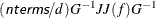
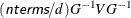
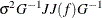
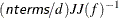
specifies one of six formulas for computing the covariance matrix. The formula that is used depends on the type of objective (MIN or LSQ) that is specified. Table 10.2 describes the valid values for this option and their corresponding formulas, where nterms is the value of the NTERMS= option and MIN, LSQ, and other symbols are defined in the section Covariance Matrix.

Table 10.2: Values of COV= Option

number	string	MIN Objective	LSQ Objective
1	M	$(\Argument{nterms}/d) G^{-1} JJ(f) G^{-1}$	$(\Argument{nterms}/d) G^{-1} V G^{-1}$
2	H	$(\Argument{nterms}/d) G^{-1}$	$\sigma ^2 G^{-1}$
3	J	$(1/d) W^{-1}$	$\sigma ^2 JJ(f)^{-1}$
4	B	$(1/d) G^{-1} W G^{-1}$	$\sigma ^2 G^{-1} JJ(f) G^{-1}$
5	E	$(\Argument{nterms}/d) JJ(f)^{-1}$	$(1/d) V^{-1}$
6	U	$(\Argument{nterms}/d) W^{-1} JJ(f) W^{-1}$	$(\Argument{nterms}/d) JJ(f)^{-1} V JJ(f)^{-1}$

For MAX type problems, the covariance matrix is converted to MIN type by using negative Hessian, Jacobian, and function values in the computation. For more information, see the section Covariance Matrix.

By default, COV=2.

COVOUT=parameter

specifies the name of the parameter that contains the output covariance matrix. Because a covariance matrix is symmetric, you should declare the covariance matrix as either a lower-triangular matrix or a square matrix with indexes starting from 1. For example:

num mycov{i in 1..N, j in 1..i};   /* a  lower triangular matrix */

or

num mycov{i in 1..N, j in 1..N};   /* a square matrix */

where N is the number of variables.

Depending on the type of output covariance matrix, the solver updates either the lower-triangular matrix or the full square matrix. If you declare the covariance matrix as neither a lower-triangular matrix nor a square matrix, or if the indexes do not start from 1, the NLP solver issues an error message. You can use the CREATE DATA statement to output the results to a SAS data set. For more information, see the section Covariance Matrix.

COVSING=covsing

specifies a threshold, $\Argument{covsing}>0$ , that determines whether to consider the eigenvalues of a matrix to be 0. The value of covsing can be any number between the machine precision and the largest positive number representable in your operating environment. The default is set internally by the algorithm. For more information, see the section Covariance Matrix.

MSINGULAR=msing

specifies a relative singularity criterion $\Argument{msing}>0$ for measuring the singularity of the Hessian and crossproduct Jacobian and their projected forms. The value of msing can be any number between machine precision and the largest positive number representable in your operating environment. The default is 1E–12. For more information, see the section Covariance Matrix.

NDF=ndf

specifies a number to be used in calculating the divisor d, which is used in calculating the covariance matrix when VARDEF=DF. The value of ndf can be any positive integer up to the largest four-byte signed integer, which is $2^{31} - 1$ . The default is the number of optimization variables in the objective function. For more information, see the section Covariance Matrix.

NTERMS=nterms

specifies a number to be used in calculating the scale factor for the covariance matrix, as shown in Table 10.2. The value of nterms can be any positive integer up to the largest four-byte signed integer, which is $2^{31} - 1$ . The default is the number of nonconstant terms in the objective function. For more information, see the section Covariance Matrix.

SIGSQ=sq

specifies a real scalar factor, $\Argument{sq} > 0$ , for computing the covariance matrix. The value of sq can be any number between the machine precision and the largest positive number representable in your operating environment. For more information, see the section Covariance Matrix.

VARDEF=DF | N

controls how the divisor d is calculated. This divisor is used in calculating the covariance matrix and approximate standard errors. The value of d also depends on the values of the NDF= and NTERMS= options, ndf and nterms, respectively, as follows:

$d = \left\{ \begin{array}{ll} \max (1,\Argument{nterms} - \Argument{ndf}) & \mbox{for VARDEF=DF} \\ \Argument{nterms} & \mbox{for VARDEF=N} \end{array} \right.$

By default, VARDEF=DF if the SIGSQ= option is not specified; otherwise, by default VARDEF=N. For more information, see the section Covariance Matrix.

Miscellaneous Option

SEED=N: specifies a positive integer to be used as the seed for generating random number sequences. You can use this option to replicate results from different runs.

Multistart Options

MULTISTART=(suboptions) MS=(suboptions)

enables multistart mode. In this mode, the local solver solves the problem from multiple starting points, possibly finding a better local minimum as a result. This option is disabled by default. For more information about multistart mode, see the section Multistart.

You can specify the following suboptions:

BNDRANGE=M

defines the range from which each variable can take values during the sampling process. This option affects only the sampling process that determines starting points for the local solver. It does not affect the bounds of the original nonlinear optimization problem. More specifically, if the ith variable $x_ i$ has lower and upper bounds $\ell _ i$ and $u_ i$ , respectively (that is, $\ell _ i \le x_ i \le u_ i$ ), then an initial point is generated by a sampling process as follows:

For each sample point x, the ith coordinate $x_ i$ is generated so that the following bounds hold, where $x_{i}^0$ is the default starting point or a specified starting point:

$\begin{array}{ll} l_ i \leq x_ i \leq u_ i & \text {if } l_ i \text { and } u_ i \text { are both finite}\\ l_ i \leq x_ i \leq l_ i + M & \text {if only } l_ i \text { is finite}\\ u_ i - M \leq x_ i \leq u_ i & \text {if only } u_ i \text { is finite}\\ x_{i}^0 - M/2 \leq x_ i \leq x_{i}^0 + M/2 & \text {otherwise}\\ \end{array}$

The default value is 200 in a shared-memory computing environment and 1,000 in a distributed computing environment.

DISTTOL= $\epsilon$

defines the tolerance by which two optimal points are considered distinct. Optimal points are considered distinct if the Euclidean distance between them is at least $\epsilon$ . The default is 1.0E–6.

LOGLEVEL=number PRINTLEVEL=number

defines the amount of information that the multistart algorithm displays in the SAS log. Table 10.3 describes the valid values of this suboption.

Table 10.3: Values for LOGLEVEL= Suboption

number	Description
0	Turns off all solver-related messages to SAS log
1	Displays multistart summary information when the algorithm terminates
2	Displays multistart iteration log and summary information when the algorithm terminates
3	Displays the same information as LOGLEVEL=2 and might display additional information

By default, LOGLEVEL=2.

MAXTIME=T

defines the maximum allowable time T (in seconds) for the NLP solver to locate the best local optimum in multistart mode. The value of the TIMETYPE= option determines the type of units that are used. The time that is specified by the MAXTIME= suboption is checked only once after the completion of the local solver. Because the local solver might be called many times, the maximum time that is specified for multistart is recommended to be greater than the maximum time specified for the local solver. If you do not specify this option, the multistart algorithm does not stop based on the amount of time elapsed.

MAXSTARTS=N

defines the maximum number of starting points to be used for local optimization. That is, there will be no more than N local optimization calls in the multistart algorithm. You can specify N to be any nonnegative integer. When N = 0, the algorithm uses the default value of this option. In a shared-memory computing environment, the default value is 100. In a distributed computing environment, the default value is a number proportional to the number of threads across all the grid nodes (usually more than 100).

Optimization Options

ALGORITHM=keyword TECHNIQUE=keyword TECH=keyword SOLVER=keyword

specifies the optimization technique to be used to solve the problem. The following keywords are valid:

INTERIORPOINT: uses a primal-dual interior point method. This technique is recommended for both small- and large-scale nonlinear optimization problems. This is the preferred solver if the problem includes a large number of inactive constraints.
ACTIVESET: uses a primal-dual active-set method. This technique is recommended for both small- and large-scale nonlinear optimization problems. This is the preferred solver if the problem includes only bound constraints or if the optimal active set can be quickly determined by the solver.
CONCURRENT (experimental): runs the INTERIORPOINT and ACTIVESET techniques in parallel, with one thread using the INTERIORPOINT technique and the other thread using the ACTIVESET technique. The solution is returned by the first method that terminates.

The default is INTERIORPOINT.

Output Options

LOGFREQ=N PRINTFREQ=N: specifies how often the iterations are displayed in the SAS log. N should be an integer between zero and the largest four-byte, signed integer, which is $2^{31} - 1$ . If $N \ge 1$ , the solver prints only those iterations that are a multiple of N. If $N = 0$ , no iteration is displayed in the log. The default value is 1.
SOLTYPE=0 $\mid$ 1: specifies whether the NLP solver should return only a solution that is locally optimal. If SOLTYPE=0, the solver returns a locally optimal solution, provided it locates one. If SOLTYPE=1, the solver returns the best feasible solution found, provided its objective value is better than that of the locally optimal solution found. The default is 1.

Solver Options

FEASTOL= $\epsilon$

defines the feasible tolerance. The solver will exit if the constraint violation is less than FEASTOL and the scaled optimality conditions are less than OPTTOL. The default is $\epsilon$ =1E–6.

HESSTYPE=FULL $\mid$ PRODUCT

specifies the type of Hessian to be used by the solver. The valid keywords for this option are FULL and PRODUCT. If HESSTYPE=FULL, the solver uses a full Hessian. If HESSTYPE=PRODUCT, the solver uses only Hessian-vector products, not the full Hessian. When the solver uses only Hessian-vector products to find a search direction, it usually uses much less memory, especially when the problem is large and the Hessian is not sparse. On the other hand, when the full Hessian is used, the algorithm can create a better preconditioner to solve the problem in less CPU time. The default is FULL.

IIS=number $\mid$ string

specifies whether the NLP solver attempts to identify a set of linear constraints and variables that form an irreducible infeasible set (IIS). Table 10.4 describes the valid values of the IIS= option.

Table 10.4: Values for IIS= Option

number	string	Description
0	OFF	Disables IIS detection.
1	ON	Enables IIS detection.

The default is OFF.

Note that when the IIS= option is enabled, all the other NLP solver options are ignored except the following:

FEASTOL=		LOGFREQ=
LOGLEVEL=		MAXITER=
MAXTIME=		TIMETYPE=

The NLP solver ignores nonlinear constraints, if any, and invokes the LP solver’s algorithm to attempt to identify an IIS. If an IIS is found, information about the infeasibilities can be found in the .status suffix values of the constraints and variables. For more information about the IIS= option, see the section Irreducible Infeasible Set of Chapter 7: The Linear Programming Solver. Also see Example 10.7 for an example that demonstrates the use of the IIS= option of the NLP solver.

MAXITER=N

specifies that the solver take at most N major iterations to determine an optimum of the NLP problem. The value of N is an integer between zero and the largest four-byte, signed integer, which is $2^{31} - 1$ . A major iteration in NLP consists of finding a descent direction and a step size along which the next approximation of the optimum resides. The default is 5,000 iterations.

MAXTIME=t

specifies an upper limit of t units of time for the optimization process, including problem generation time and solution time. The value of the TIMETYPE= option determines the type of units used. If you do not specify the MAXTIME= option, the solver does not stop based on the amount of time elapsed. The value of t can be any positive number; the default value is the positive number that has the largest absolute value that can be represented in your operating environment.

OBJLIMIT=M

specifies an upper limit on the magnitude of the objective value. For a minimization problem, the algorithm terminates when the objective value becomes less than –M; for a maximization problem, the algorithm stops when the objective value exceeds M. The algorithm stopping implies that either the problem is unbounded or the algorithm diverges. If optimization were allowed to continue, numerical difficulty might be encountered. The default is M=1E $+$ 20. The minimum acceptable value of M is 1E $+$ 8. If the specified value of M is less than 1E $+$ 8, the value is reset to the default value 1E $+$ 20.

OPTTOL= $\epsilon$ RELOPTTOL= $\epsilon$

defines the measure by which you can decide whether the current iterate is an acceptable approximation of a local minimum. The value of this option is a positive real number. The NLP solver determines that the current iterate is a local minimum when the norm of the scaled vector of the optimality conditions is less than $\epsilon$ and the true constraint violation is less than FEASTOL. The default is $\epsilon$ =1E–6.

TIMETYPE=number $\mid$ string

specifies the units of time used by the MAXTIME= option and reported by the PRESOLVE_TIME and SOLUTION_TIME terms in the _OROPTMODEL_ macro variable. Table 10.5 describes the valid values of the TIMETYPE= option.

Table 10.5: Values for TIMETYPE= Option

number	string	Description
0	CPU	Specifies units of CPU time
1	REAL	Specifies units of real time

The "Optimization Statistics" table, an output of PROC OPTMODEL if you specify PRINTLEVEL=2 in the PROC OPTMODEL statement, also includes the same time units for Presolver Time and Solver Time. The other times (such as Problem Generation Time) in the "Optimization Statistics" table are also in the same units.

The default value of the TIMETYPE= option depends on various options. When the solver is used with distributed or multithreaded processing, then by default TIMETYPE= REAL. Otherwise, by default TIMETYPE= CPU. Table 10.6 describes the detailed logic for determining the default; the first context in the table that applies determines the default value. The NTHREADS= and NODES= options are specified in the PERFORMANCE statement of the OPTMODEL procedure. For more information about the NTHREADS= and NODES= options, see the section PERFORMANCE Statement in Chapter 4: Shared Concepts and Topics.

Table 10.6: Default Value for TIMETYPE= Option

Context	Default
Solver is invoked in an OPTMODEL COFOR loop	REAL
NODES= value is nonzero for multistart mode	REAL
NTHREADS= value is greater than 1	REAL
NTHREADS= 1	CPU

The Nonlinear Programming Solver