The Nonlinear Programming Solver
- Overview
-
Getting Started

-
Syntax
-
Details
-
ExamplesSolving Highly Nonlinear Optimization ProblemsSolving Unconstrained and Bound-Constrained Optimization ProblemsSolving NLP Problems with Range ConstraintsSolving Large-Scale NLP ProblemsSolving NLP Problems That Have Several Local MinimaMaximum Likelihood Weibull EstimationFinding an Irreducible Infeasible Set
- References
Active-Set Method
Active-set methods differ from interior point methods in that no barrier term is used to ensure that the algorithm remains interior with respect to the inequality constraints. Instead, attempts are made to learn the true active set. For simplicity, use the same initial slack formulation used by the interior point method description,
![\[ \begin{array}{ll} \displaystyle \mathop {\textrm{minimize}}& f(x) \\ \textrm{subject to}& g_{i}(x) - s_{i} = 0, i \in \mathcal{I} \\ & s \ge 0 \end{array} \]](images/ormpug_nlpsolver0095.png)
where  is the vector of slack variables, which are required to be nonnegative. Begin by absorbing the equality constraints as before
into a penalty function, but keep the slack bound constraints explicitly:
is the vector of slack variables, which are required to be nonnegative. Begin by absorbing the equality constraints as before
into a penalty function, but keep the slack bound constraints explicitly:
![\[ \begin{array}{ll} \displaystyle \mathop {\textrm{minimize}}& \mathcal{M}(x,s) = f(x) + \dfrac {1}{2\mu }\| g(x) -s\| _2^2 \\ \textrm{subject to}& s \ge 0 \end{array} \]](images/ormpug_nlpsolver0115.png)
where  is a positive parameter. Given a solution pair
  for the preceding problem, you can define the active-set projection matrix P as follows:
![\[ P_{ij} = \left\{ \begin{array}{cl} 1 & \text {if } i=j \text { and } s_ i(\mu ) = 0 \\ 0 & \text {otherwise.} \end{array} \right. \]](images/ormpug_nlpsolver0117.png)
Then  is also a solution of the equality constraint subproblem:
![\[ \begin{array}{ll} \displaystyle \mathop {\textrm{minimize}}& \mathcal{M}(x,s) = f(x) + \dfrac {1}{2\mu }\| g(x) -s\| _2^2 \\ \textrm{subject to}& Ps = 0. \end{array} \]](images/ormpug_nlpsolver0119.png)
The minimizer of the preceding subproblem must be a stationary point of the Lagrangian function
![\[ \mathcal{L}^{\mu }(x,s,z) = f(x) + \dfrac {1}{2\mu }\| g(x) -s\| _2^2 - z^{T} Ps \]](images/ormpug_nlpsolver0120.png)
which gives the optimality equations
![\[ \begin{array}{lclclc} \nabla _ x \mathcal{L}^{\mu }(x,s,z) & =& \nabla f(x) - J(x)^{T} y & =& 0 \\ \nabla _ s \mathcal{L}^{\mu }(x,s,z) & =& y - P^{T}z & =& 0 \\ & =& Ps & =& 0 \end{array} \]](images/ormpug_nlpsolver0121.png)
where 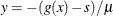 . Using the second equation, you can simplify the preceding equations to get the following optimality conditions for the bound-constrained
penalty subproblem:
. Using the second equation, you can simplify the preceding equations to get the following optimality conditions for the bound-constrained
penalty subproblem:
![\[ \begin{array}{lclclc} \nabla f(x) - J(x)^{T} P^{T}z & =& 0 \\ P(g(x) -s) + \mu z & =& 0 \\ Ps & =& 0 \end{array} \]](images/ormpug_nlpsolver0123.png)
Using the third equation directly, you can reduce the system further to
![\[ \begin{array}{lclclc} \nabla f(x) - J(x)^{T} P^{T}z & =& 0 \\ P g(x) + \mu z & =& 0 \\ \end{array} \]](images/ormpug_nlpsolver0124.png)
At iteration k, the primal-dual active-set algorithm approximately solves the preceding system by using Newton’s method. The Newton system is
![\[ \left[\begin{array}{ccc} H_{\mathcal{L}}(x^{k}, z^{k}) & -J_{\mathcal A}^\mr {T} \\ J_{\mathcal A} & \mu I \end{array}\right] \left[\begin{array}{c} \Delta x^{k} \\ \Delta z^{k} \end{array}\right] = - \left[\begin{array}{c} \nabla _{x} f(x^{k}) - J_{\mathcal A}^\mr {T} z\\ Pg(x^{k}) + \mu z^{k} \end{array}\right] \]](images/ormpug_nlpsolver0125.png)
where  and
and  denotes the Hessian of the Lagrangian function
  . The solution
  of the Newton system provides a direction to move from the current iteration
  to the next,
![\[ (x^{k+1}, z^{k+1}) = (x^{k},z^{k}) + \alpha (\Delta x^{k}, \Delta z^{k}) \]](images/ormpug_nlpsolver0129.png)
where  is the step length along the Newton direction. The corresponding slack variable update
  is defined as the solution to the following subproblem whose solution can be computed analytically:
![\[ \begin{array}{ll} \displaystyle \mathop {\textrm{minimize}}& \mathcal{M}(x^{k+1},s) = f(x) + \dfrac {1}{2\mu }\| g(x^{k+1}) -s\| _2^2 \\ \textrm{subject to}& s \ge 0 \end{array} \]](images/ormpug_nlpsolver0131.png)
The step length is then determined in a similar manner to the preceding interior point approach. At each iteration, the definition of the
active-set projection matrix P is updated with respect to the new value of the constraint function  . For large-scale NLP, the computational bottleneck typically arises in seeking to solve the Newton system. Thus active-set
methods can achieve substantial computational savings when the size of
. For large-scale NLP, the computational bottleneck typically arises in seeking to solve the Newton system. Thus active-set
methods can achieve substantial computational savings when the size of  is much smaller than
  ; however, convergence can be slow if the active-set estimate changes combinatorially. Further, the active-set algorithm is
often the superior algorithm when only bound constraints are present. In practice, both the interior point and active-set
approach incorporate more sophisticated merit functions than those described in the preceding sections; however, their description
is beyond the scope of this document. See Gill and Robinson (2010) for further reading.
; however, convergence can be slow if the active-set estimate changes combinatorially. Further, the active-set algorithm is
often the superior algorithm when only bound constraints are present. In practice, both the interior point and active-set
approach incorporate more sophisticated merit functions than those described in the preceding sections; however, their description
is beyond the scope of this document. See Gill and Robinson (2010) for further reading.