The Decomposition Algorithm
- Overview
-
Getting Started

-
SyntaxDecomposition Algorithm Options in the PROC OPTLP Statement or the SOLVE WITH LP Statement in PROC OPTMODELDecomposition Algorithm Options in the PROC OPTMILP Statement or the SOLVE WITH MILP Statement in PROC OPTMODELDECOMP StatementDECOMP_MASTER StatementDECOMP_MASTER_IP StatementDECOMP_SUBPROB Statement
-
Details
-
ExamplesMulticommodity Flow Problem and METHOD=NETWORKGeneralized Assignment ProblemBlock-Diagonal Structure and METHOD=CONCOMP in Single-Machine ModeBlock-Diagonal Structure and METHOD=CONCOMP in Distributed ModeBlock-Angular Structure and METHOD=AUTOBin Packing ProblemResource Allocation ProblemVehicle Routing ProblemATM Cash Management in Single-Machine ModeATM Cash Management in Distributed ModeKidney Donor Exchange and METHOD=SET
- References
Example 15.8 Vehicle Routing Problem
The vehicle routing problem (VRP) finds a minimum-cost routing of a fixed number of vehicles to service the demands of a set
of customers. Define a set 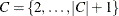 of customers, and a demand,
  , for each customer c. Let
  be the set of nodes, including the vehicle depot, which are designated as node
  . Let
. Let  be the set of arcs, V be the set of vehicles (each of which has capacity L), and
  be the travel time from node i to node j.
Let  be a binary variable that, if set to 1, indicates that node i is visited by vehicle k. Let
  be a binary variable that, if set to 1, indicates that arc
  is traversed by vehicle k, and let
  be a continuous variable that denotes the amount of product (flow) on arc that is carried by vehicle k.
A VRP can be formulated as a MILP as follows:
In this formulation, the Assignment constraints ensure that each customer is serviced by at least one vehicle. The objective function ensures that there exists an optimal solution that never assigns a customer to more than one vehicle. The LeaveNode and EnterNode constraints enforce the condition that if node i is visited by vehicle k, then vehicle k must use exactly one arc that enters node i and one arc that leaves node i. Conversely, if node i is not visited by vehicle k, then no arcs that enter or leave node i can be used by vehicle k. The FlowBalance constraints define flow conservation at each node for each vehicle. That is, if a node i is visited by vehicle k, then the amount of product from vehicle k that enters and leaves that node must equal the demand at that node. Conversely, if node i is not visited by vehicle k, then the amount of product from vehicle k that enters and leaves that node must be 0. The VehicleCapacity constraints enforce the condition that the amount of product in each vehicle must always be less than or equal to the vehicle capacity L. Finally, the Depot constraints enforce the condition that each vehicle must start and end at the depot node.
In this formulation, the vehicle identifier is arbitrary. Consider a decomposition by vehicle, where the Assignment constraints form the master problem and all other constraints form identical routing subproblems. As described in the section Special Case: Identical Blocks and Ryan-Foster Branching, this is a situation in which an aggregate formulation can greatly improve performance by reducing symmetry. Because you know that there exists an optimal solution that satisfies the master Assignment constraints at equality, you can force the use of Ryan-Foster branching by specifying the option VARSEL=RYANFOSTER.
VRPLIB, located at http://www.coin-or.org/SYMPHONY/branchandcut/VRP/data/index.htm, is a set of benchmark instances of the VRP. The following data set, vrpdata, represents an instance from VRPLIB that has 22 nodes and eight vehicles (P-n22-k8.vrp), which was originally described in
Augerat et al. (1995). The data set lists each node, its coordinates, and its demand.
/* number of vehicles available */
%let num_vehicles = 8;
/* capacity of each vehicle */
%let capacity = 3000;
/* node, x coordinate, y coordinate, demand */
data vrpdata;
   input node x y demand;
   datalines;
1  145 215    0
2  151 264 1100
3  159 261  700
4  130 254  800
5  128 252 1400
6  163 247 2100
7  146 246  400
8  161 242  800
9  142 239  100
10 163 236  500
11 148 232  600
12 128 231 1200
13 156 217 1300
14 129 214 1300
15 146 208  300
16 164 208  900
17 141 206 2100
18 147 193 1000
19 164 193  900
20 129 189 2500
21 155 185 1800
22 139 182  700
;
The following PROC OPTMODEL statements read in the data, declare the optimization model, and use the decomposition algorithm to solve it:
proc optmodel;
   /* read the node location and demand data */
   set NODES;
   num x {NODES};
   num y {NODES};
   num demand {NODES};
   num capacity = &capacity;
   num num_vehicles = &num_vehicles;
   read data vrpdata into NODES=[node] x y demand;
   set ARCS = {i in NODES, j in NODES: i ne j};
   set VEHICLES = 1..num_vehicles;

   /* define the depot as node 1 */
   num depot = 1;

   /* define the arc cost as the rounded Euclidean distance */
   num cost {<i,j> in ARCS} = round(sqrt((x[i]-x[j])^2 + (y[i]-y[j])^2));

   /* Flow[i,j,k] is the amount of demand carried on arc (i,j) by vehicle k */
   var Flow {ARCS, VEHICLES} >= 0 <= capacity;
   /* UseNode[i,k] = 1, if and only if node i is serviced by vehicle k */
   var UseNode {NODES, VEHICLES} binary;
   /* UseArc[i,j,k] = 1, if and only if arc (i,j) is traversed by vehicle k */
   var UseArc {ARCS, VEHICLES} binary;

   /* minimize the total distance traversed */
   min TotalCost = sum {<i,j> in ARCS, k in VEHICLES} cost[i,j] * UseArc[i,j,k];

   /* each non-depot node must be serviced by at least one vehicle */
   con Assignment {i in NODES diff {depot}}:
      sum {k in VEHICLES} UseNode[i,k] >= 1;

   /* each vehicle must start at the depot node */
   for{k in VEHICLES} fix UseNode[depot,k] = 1;

   /* some vehicle k traverses an arc that leaves node i
      if and only if UseNode[i,k] = 1 */
   con LeaveNode {i in NODES, k in VEHICLES}:
      sum {<(i),j> in ARCS} UseArc[i,j,k] = UseNode[i,k];

   /* some vehicle k traverses an arc that enters node i
      if and only if UseNode[i,k] = 1 */
   con EnterNode {i in NODES, k in VEHICLES}:
      sum {<j,(i)> in ARCS} UseArc[j,i,k] = UseNode[i,k];

   /* the amount of demand supplied by vehicle k to node i must equal demand
      if UseNode[i,k] = 1; otherwise, it must equal 0 */
   con FlowBalance {i in NODES diff {depot}, k in VEHICLES}:
       sum {<j,(i)> in ARCS} Flow[j,i,k] - sum {<(i),j> in ARCS} Flow[i,j,k]
       = demand[i] * UseNode[i,k];

   /* if UseArc[i,j,k] = 1, then the flow on arc (i,j) must be at most capacity
      if UseArc[i,j,k] = 0, then no flow is allowed on arc (i,j) */
   con VehicleCapacity {<i,j> in ARCS, k in VEHICLES}:
      Flow[i,j,k] <= Flow[i,j,k].ub * UseArc[i,j,k];

   /* decomp by vehicle */
   for {i in NODES, k in VEHICLES} do;
      LeaveNode[i,k].block = k;
      EnterNode[i,k].block = k;
   end;
   for {i in NODES diff {depot}, k in VEHICLES} FlowBalance[i,k].block = k;
   for {<i,j> in ARCS, k in VEHICLES} VehicleCapacity[i,j,k].block = k;

   /* solve using decomp (aggregate formulation) */
   solve with MILP / varsel=ryanfoster decomp=(logfreq=20);
The following OPTMODEL statements create node and edge data for the optimal routing:
   /* create solution data set */
   str color {k in VEHICLES} =
      ['red' 'green' 'blue' 'black' 'orange' 'gray' 'maroon' 'purple'];
   create data node_data from [i] x y;
   create data edge_data from [i j k]=
      {<i,j> in ARCS, k in VEHICLES: UseArc[i,j,k].sol > 0.5}
      x1=x[i] y1=y[i] x2=x[j] y2=y[j] linecolor=color[k];
quit;
The solution summary is displayed in Output 15.8.1.
Output 15.8.1: Solution Summary
| Solution Summary | |
|---|---|
| Solver | MILP |
| Algorithm | Decomposition |
| Objective Function | TotalCost |
| Solution Status | Optimal |
| Objective Value | 603 |
| Relative Gap | 0 |
| Absolute Gap | 0 |
| Primal Infeasibility | 7.730705E-12 |
| Bound Infeasibility | 9.325873E-15 |
| Integer Infeasibility | 9.325873E-15 |
| Best Bound | 603 |
| Nodes | 1 |
| Iterations | 70 |
| Presolve Time | 0.17 |
| Solution Time | 87.55 |
The iteration log is displayed in Output 15.8.2.
Output 15.8.2: Log
| NOTE: There were 22 observations read from the data set WORK.VRPDATA. |
| NOTE: Problem generation will use 4 threads. |
| NOTE: The problem has 7568 variables (0 free, 8 fixed). |
| NOTE: The problem has 3872 binary and 0 integer variables. |
| NOTE: The problem has 4237 linear constraints (3696 LE, 520 EQ, 21 GE, 0 range). |
| NOTE: The problem has 22528 linear constraint coefficients. |
| NOTE: The problem has 0 nonlinear constraints (0 LE, 0 EQ, 0 GE, 0 range). |
| NOTE: The MILP presolver value AUTOMATIC is applied. |
| NOTE: The MILP presolver removed 8 variables and 0 constraints. |
| NOTE: The MILP presolver removed 16 constraint coefficients. |
| NOTE: The MILP presolver modified 0 constraint coefficients. |
| NOTE: The presolved problem has 7560 variables, 4237 constraints, and 22512 constraint |
| coefficients. |
| NOTE: The MILP solver is called. |
| NOTE: The Decomposition algorithm is used. |
| NOTE: The Decomposition algorithm is executing in single-machine mode. |
| NOTE: The DECOMP method value USER is applied. |
| NOTE: All blocks are identical and the master model is set covering. |
| WARNING: The master model is not a set partitioning and VARSEL=RYANFOSTER. The objective |
| function must ensure that there exists at least one optimal solution that fulfills all |
| of the master constraints at equality. |
| NOTE: The Decomposition algorithm is using an aggregate formulation and Ryan-Foster branching. |
| NOTE: The number of block threads has been reduced to 1 threads. |
| NOTE: The problem has a decomposable structure with 8 blocks. The largest block covers 12.44% |
| of the constraints in the problem. |
| NOTE: The decomposition subproblems cover 7560 (100%) variables and 4216 (99.5%) constraints. |
| NOTE: The deterministic parallel mode is enabled. |
| NOTE: The Decomposition algorithm is using up to 4 threads. |
| Iter Best Master Best LP IP CPU Real |
| Bound Objective Integer Gap Gap Time Time |
| NOTE: Starting phase 1. |
| 1 0.0000 20.0000 . 2.00e+01 . 1 1 |
| 20 0.0000 0.7500 . 7.50e-01 . 6 5 |
| 25 0.0000 0.0000 . 0.00% . 8 7 |
| NOTE: Starting phase 2. |
| . 112.0000 969.0000 969.0000 765.18% 765.18% 8 7 |
| 29 112.0000 884.9730 907.0000 690.15% 709.82% 9 8 |
| 32 112.0000 747.0000 747.0000 566.96% 566.96% 21 14 |
| 39 186.0829 684.8000 747.0000 268.01% 301.43% 40 26 |
| . 186.0829 656.5000 747.0000 252.80% 301.43% 40 26 |
| 40 186.0829 656.5000 747.0000 252.80% 301.43% 42 27 |
| 41 249.3439 656.5000 747.0000 163.29% 199.59% 44 29 |
| 42 278.7811 656.5000 747.0000 135.49% 167.95% 48 31 |
| 44 297.0744 656.5000 747.0000 120.99% 151.45% 49 33 |
| 45 338.7579 656.5000 747.0000 93.80% 120.51% 53 36 |
| 47 358.8263 656.5000 747.0000 82.96% 108.18% 57 39 |
| 52 455.9563 648.1538 660.0000 42.15% 44.75% 69 48 |
| 56 499.1319 616.4444 660.0000 23.50% 32.23% 77 54 |
| 59 531.4382 610.1538 660.0000 14.81% 24.19% 91 60 |
| 60 531.4382 606.6923 660.0000 14.16% 24.19% 95 63 |
| 62 569.3333 604.0000 604.0000 6.09% 6.09% 104 66 |
| 63 572.0000 604.0000 604.0000 5.59% 5.59% 113 70 |
| 67 597.1667 603.8333 604.0000 1.12% 1.14% 140 80 |
| 69 597.1667 603.0000 603.0000 0.98% 0.98% 147 84 |
| 70 603.0000 603.0000 603.0000 0.00% 0.00% 156 87 |
| Node Active Sols Best Best Gap CPU Real |
| Integer Bound Time Time |
| 0 0 7 603.0000 603.0000 0.00% 156 87 |
| NOTE: The Decomposition algorithm used 4 threads. |
| NOTE: The Decomposition algorithm time is 87.36 seconds. |
| NOTE: Optimal. |
| NOTE: Objective = 603. |
| NOTE: The data set WORK.NODE_DATA has 22 observations and 3 variables. |
| NOTE: The data set WORK.EDGE_DATA has 29 observations and 8 variables. |
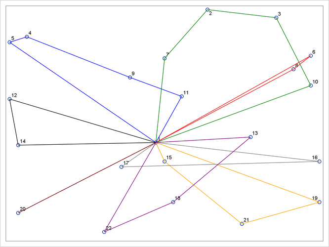
The following DATA step and call to PROC SGPLOT generate a plot of the optimal routing. The plot is displayed in Output 15.8.3.
data sganno(drop=i j);
   retain drawspace "datavalue" linethickness 1;
   set edge_data;
   function = 'line';
run;

proc sgplot data=node_data sganno=sganno;
   scatter x=x y=y / datalabel=i;
   xaxis display=none;
   yaxis display=none;
run;
Output 15.8.3: Optimal Routing