The Decomposition Algorithm
- Overview
-
Getting Started

-
SyntaxDecomposition Algorithm Options in the PROC OPTLP Statement or the SOLVE WITH LP Statement in PROC OPTMODELDecomposition Algorithm Options in the PROC OPTMILP Statement or the SOLVE WITH MILP Statement in PROC OPTMODELDECOMP StatementDECOMP_MASTER StatementDECOMP_MASTER_IP StatementDECOMP_SUBPROB Statement
-
Details
-
ExamplesMulticommodity Flow Problem and METHOD=NETWORKGeneralized Assignment ProblemBlock-Diagonal Structure and METHOD=CONCOMP in Single-Machine ModeBlock-Diagonal Structure and METHOD=CONCOMP in Distributed ModeBlock-Angular Structure and METHOD=AUTOBin Packing ProblemResource Allocation ProblemVehicle Routing ProblemATM Cash Management in Single-Machine ModeATM Cash Management in Distributed ModeKidney Donor Exchange and METHOD=SET
- References
Example 15.6 Bin Packing Problem
The bin packing problem (BPP) finds the minimum number of capacitated bins that are needed to store a set of products of varying
size. Define a set P of products, their sizes  , and a set
  of candidate bins, each having capacity C. Let
  be a binary variable that, if set to 1, indicates that product p is assigned to bin b. In addition, let
  be a binary variable that, if set to 1, indicates that bin b is used.
A BPP can be formulated as a MILP as follows:
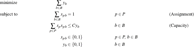
In this formulation, the Assignment constraints ensure that each product is assigned to exactly one bin. The Capacity constraints
ensure that the capacity restrictions are met for each bin. In addition, these constraints enforce the condition that if any
product is assigned to bin b, then must be positive.
In this formulation, the bin identifier is arbitrary. For example, in any solution, the assignments to bin 1 can be swapped with the assignments to bin 2 without affecting feasibility or the objective value. Consider a decomposition by bin, where the Assignment constraints form the master problem and the Capacity constraints form identical subproblems. As described in the section Special Case: Identical Blocks and Ryan-Foster Branching, this is a situation in which an aggregate formulation and Ryan-Foster branching can greatly improve performance by reducing symmetry.
Consider a series of University of North Carolina basketball games that are recorded on a DVR. The following data set, dvr, provides the name of each game in the column opponent and the size of that game in gigabytes (GB) as it resides on the DVR in the column size:
/* game, size (in GBs) */
data dvr;
   input opponent $ size;
   datalines;
Clemson  1.36
Clemson2 1.97
Duke     2.76
Duke2    2.52
FSU      2.56
FSU2     2.34
GT       1.49
GT2      1.12
IN       1.45
KY       1.42
Loyola   1.42
MD       1.33
MD2      2.71
Miami    1.22
NCSU     2.52
NCSU2    2.54
UConn    1.25
VA       2.33
VA2      2.48
VT       1.41
Vermont  1.28
WM       1.25
WM2      1.23
Wake     1.61
;
The goal is to use the fewest DVDs on which to store the games for safekeeping. Each DVD can hold 4.38GB reforded data. The problem can be formulated as a bin packing problem and solved by using PROC OPTMODEL and the decomposition algorithm. The following PROC OPTMODEL statements read in the data, declare the optimization model, and use the decomposition algorithm to solve it:
proc optmodel;
   /* read the product and size data */
   set <str> PRODUCTS;
   num size {PRODUCTS};
   read data dvr into PRODUCTS=[opponent] size;

   /* 4.38 GBs per DVD */
   num binsize = 4.38;

   /* the number of products is a trivial upper bound on the
      number of bins needed */
   num upperbound init card(PRODUCTS);
   set BINS = 1..upperbound;

   /* Assign[p,b] = 1, if product p is assigned to bin b */
   var Assign {PRODUCTS, BINS} binary;
   /* UseBin[b] = 1, if bin b is used */
   var UseBin {BINS} binary;

   /* minimize number of bins used */
   min Objective = sum {b in BINS} UseBin[b];

   /* assign each product to exactly one bin */
   con Assignment {p in PRODUCTS}:
      sum {b in BINS} Assign[p,b] = 1;

   /* Capacity constraint on each bin (and definition of UseBin) */
   con Capacity {b in BINS}:
      sum {p in PRODUCTS} size[p] * Assign[p,b] <= binsize * UseBin[b];

   /* decompose by bin (subproblem is a knapsack problem) */
   for {b in BINS} Capacity[b].block = b;

   /* solve using decomp (aggregate formulation) */
   solve with milp / decomp;
The following OPTMODEL statements create a sequential numbering of the bins and then output to the data set dvd the optimal assignments of games to bins:
   /* create a map from arbitrary bin number to sequential bin number */
   num binId init 1;
   num binMap {BINS};
   for {b in BINS: UseBin[b].sol > 0.5} do;
      binMap[b] = binId;
      binId     = binId + 1;
   end;

   /* create map of product to bin from solution */
   num bin {PRODUCTS};
   for {p in PRODUCTS} do;
      for {b in BINS: Assign[p,b].sol > 0.5} do;
         bin[p] = binMap[b];
         leave;
      end;
   end;

   /* create solution data */
   create data dvd from [product] bin size;
quit;
The solution summary is displayed in Output 15.6.1.
Output 15.6.1: Solution Summary
| Solution Summary | |
|---|---|
| Solver | MILP |
| Algorithm | Decomposition |
| Objective Function | Objective |
| Solution Status | Optimal |
| Objective Value | 11 |
| Relative Gap | 0 |
| Absolute Gap | 0 |
| Primal Infeasibility | 0 |
| Bound Infeasibility | 0 |
| Integer Infeasibility | 0 |
| Best Bound | 11 |
| Nodes | 1 |
| Iterations | 18 |
| Presolve Time | 0.02 |
| Solution Time | 0.25 |
The iteration log is displayed in Output 15.6.2.
Output 15.6.2: Log
| NOTE: There were 24 observations read from the data set WORK.DVR. |
| NOTE: Problem generation will use 4 threads. |
| NOTE: The problem has 600 variables (0 free, 0 fixed). |
| NOTE: The problem has 600 binary and 0 integer variables. |
| NOTE: The problem has 48 linear constraints (24 LE, 24 EQ, 0 GE, 0 range). |
| NOTE: The problem has 1176 linear constraint coefficients. |
| NOTE: The problem has 0 nonlinear constraints (0 LE, 0 EQ, 0 GE, 0 range). |
| NOTE: The MILP presolver value AUTOMATIC is applied. |
| NOTE: The MILP presolver removed 0 variables and 0 constraints. |
| NOTE: The MILP presolver removed 0 constraint coefficients. |
| NOTE: The MILP presolver modified 0 constraint coefficients. |
| NOTE: The presolved problem has 600 variables, 48 constraints, and 1176 constraint coefficients. |
| NOTE: The MILP solver is called. |
| NOTE: The Decomposition algorithm is used. |
| NOTE: The Decomposition algorithm is executing in single-machine mode. |
| NOTE: The DECOMP method value USER is applied. |
| NOTE: All blocks are identical and the master model is set partitioning. |
| NOTE: The Decomposition algorithm is using an aggregate formulation and Ryan-Foster branching. |
| NOTE: The number of block threads has been reduced to 1 threads. |
| NOTE: The problem has a decomposable structure with 24 blocks. The largest block covers 2.083% |
| of the constraints in the problem. |
| NOTE: The decomposition subproblems cover 600 (100%) variables and 24 (50%) constraints. |
| NOTE: The deterministic parallel mode is enabled. |
| NOTE: The Decomposition algorithm is using up to 4 threads. |
| Iter Best Master Best LP IP CPU Real |
| Bound Objective Integer Gap Gap Time Time |
| . 0.0000 11.0000 11.0000 1.10e+01 1.10e+01 0 0 |
| . 0.0000 11.0000 11.0000 1.10e+01 1.10e+01 0 0 |
| 10 0.0000 11.0000 11.0000 1.10e+01 1.10e+01 0 0 |
| 12 3.0000 11.0000 11.0000 266.67% 266.67% 0 0 |
| 18 11.0000 11.0000 11.0000 0.00% 0.00% 0 0 |
| Node Active Sols Best Best Gap CPU Real |
| Integer Bound Time Time |
| 0 0 2 11.0000 11.0000 0.00% 0 0 |
| NOTE: The Decomposition algorithm used 4 threads. |
| NOTE: The Decomposition algorithm time is 0.23 seconds. |
| NOTE: Optimal. |
| NOTE: Objective = 11. |
| NOTE: The data set WORK.DVD has 24 observations and 3 variables. |
The following call to PROC SORT sorts the assignments by bin:
proc sort data=dvd;
   by bin;
run;
The optimal assignments from the output data set dvd are displayed in Figure 15.7.
Figure 15.7: Optimal Assignment of Games to DVDs
In this example, the objective function ensures that there exists an optimal solution that never assigns a product to more than one bin. Therefore, you could instead model the Assignment constraint as an inequality rather than an equality. In this case, the best performance would come from forcing the use of an aggregate formulation and Ryan-Foster branching by specifying the option VARSEL=RYANFOSTER. An example of doing this is shown in Example 15.8.