The Decomposition Algorithm
- Overview
-
Getting Started

-
SyntaxDecomposition Algorithm Options in the PROC OPTLP Statement or the SOLVE WITH LP Statement in PROC OPTMODELDecomposition Algorithm Options in the PROC OPTMILP Statement or the SOLVE WITH MILP Statement in PROC OPTMODELDECOMP StatementDECOMP_MASTER StatementDECOMP_MASTER_IP StatementDECOMP_SUBPROB Statement
-
Details
-
ExamplesMulticommodity Flow Problem and METHOD=NETWORKGeneralized Assignment ProblemBlock-Diagonal Structure and METHOD=CONCOMP in Single-Machine ModeBlock-Diagonal Structure and METHOD=CONCOMP in Distributed ModeBlock-Angular Structure and METHOD=AUTOBin Packing ProblemResource Allocation ProblemVehicle Routing ProblemATM Cash Management in Single-Machine ModeATM Cash Management in Distributed ModeKidney Donor Exchange and METHOD=SET
- References
Example 15.7 Resource Allocation Problem
This example describes a model for selecting tasks to be run on a shared resource (Gamrath 2010). Consider a set I of tasks and a resource capacity C. Each item  has a profit
  , a resource utilization level
  , a starting period
  , and an ending period
  . The time horizon that is considered is from the earliest starting time to the latest ending time of all tasks. With each
task, associate a binary variable
. The time horizon that is considered is from the earliest starting time to the latest ending time of all tasks. With each
task, associate a binary variable  , which, if set to 1, indicates that the task is running from its start time until just before its end time. A task consumes
capacity if it is running. The goal is to select which tasks to run in order to maximize profit while not exceeding the shared
resource capacity. Let
, which, if set to 1, indicates that the task is running from its start time until just before its end time. A task consumes
capacity if it is running. The goal is to select which tasks to run in order to maximize profit while not exceeding the shared
resource capacity. Let  define the set of start times for all tasks, and let
 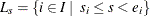 define the set of tasks that are running at each start time
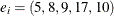
  . You can model the problem as a mixed integer linear programming problem as follows:
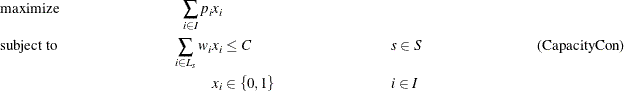
In this formulation, CapacityCon constraints ensure that the running tasks do not exceed the resource capacity. To illustrate,
consider the following five-task example with data: 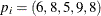 ,
,  ,
,  ,
,  , and
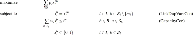
, and  . The formulation leads to a constraint matrix that has a staircase structure that is determined by tasks coming online and offline:
![\[ \begin{array}{rlllllllllll} \mbox{maximize} & 6 x_1 & + & 8 x_2 & + & 5 x_3 & + & 9 x_4 & + & 8 x_5 \\ \mbox{subject to} & 8 x_1 & & & & & & & & & \leq & 10 \\ & 8 x_1 & + & 5 x_2 & & & & & & & \leq & 10 \\ & & & 5 x_2 & + & 3 x_3 & & & & & \leq & 10 \\ & & & 5 x_2 & + & 3 x_3 & + & 4 x_4 & & & \leq & 10 \\ & & & & + & 3 x_3 & + & 4 x_4 & + & 3 x_5 & \leq & 10 \\ & \multicolumn{11}{l}{x_ i \in \{ 0,1\} \quad i \in I}\\ \end{array} \]](images/ormpug_decomp0088.png)
Lagrangian Decomposition
This formulation clearly has no decomposable structure. However, you can use a common modeling technique known as Lagrangian decomposition to bring the model into block-angular form. Lagrangian decomposition works by first partitioning the constraints into blocks. Then, each original variable is split into multiple copies of itself, one copy for each block in which the variable has a nonzero coefficient in the constraint matrix. Constraints are added to enforce the equality of each copy of the original variable. Then, you can write the original constraints in block-angular form by using the duplicate variables.
To apply Lagrangian decomposition to the resource allocation problem, define a set B of blocks and let  define the set of start times for a given block b, such that
  . Given this partition of start times, let
  define the set of blocks in which task is scheduled to be running. Now, for each task , define duplicate variables
  for each
  . Let
. Let  define the minimum block index for each class of variable that represents task i. You can now model the problem in block-angular form as follows:
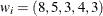
In this formulation, the LinkDupVarsCon constraints ensure that the duplicate variables are equal to the original variables. Now, the five-task example has been transformed from a staircase structure to a block-angular structure:
![\[ \begin{array}{r*{18}{r}} \mbox{maximize} & 6 x_1^1 & + & 8 x_2^1 & + & & & 5 x_3^2 & + & 9 x_4^2 & + & & & & & 8 x_5^3 \\ \mbox{subject to} & & & x_2^1 & - & x_2^2 & & & & & & & & & & & = & 0 \\ & & & & & & & x_3^2 & - & & & x_3^3 & & & & & = & 0 \\ & & & & & & & & & x_4^2 & & & - & x_4^3 & & & = & 0 \\ & 8 x_1^1 & & & & & & & & & & & & & & & \leq & 10 \\ & 8 x_1^1 & + & 5 x_2^1 & & & & & & & & & & & & & \leq & 10 \\ & & & & & 5 x_2^2 & + & 3 x_3^2 & & & & & & & & & \leq & 10 \\ & & & & & 5 x_2^2 & + & 3 x_3^2 & + & 4 x_4^2 & & & & & & & \leq & 10 \\ & & & & & & & & & & & 3 x_3^3 & + & 4 x_4^3 & + & 3 x_5^3 & \leq & 10 \\ & \multicolumn{11}{l}{x_ i^ b \in \{ 0,1\} \quad i \in I, \ b \in B_ i}\\ \end{array} \]](images/ormpug_decomp0096.png)
To see how to apply Lagrangian decomposition
in PROC OPTMODEL, consider the data set TaskData from Caprara, Furini, and Malaguti (2010), which consists of  2,916 tasks:
data TaskData;
   input profit weight start end;
   datalines;
99 92 1 9
56 30 1 3
39 73 1 20
86 76 1 9
...
24 94 768 769
95 40 768 769
66 17 768 769
18 48 768 769
97 23 768 769
;
Using the MILP Solver Directly in PROC OPTMODEL
The following PROC OPTMODEL statements read in the data and solve the original staircase formulation by calling the MILP solver directly:
%macro SetupData(task_data=, capacity=);
   set TASKS;
   num capacity=&capacity;
   num profit{TASKS}, weight{TASKS}, start{TASKS}, end{TASKS};

   read data &task_data into TASKS=[_n_] profit weight start end;
   /* the set of start times */

   set STARTS = setof{i in TASKS} start[i];
   /* the set of tasks i that are active at a given start time s */
   set TASKS_START{s in STARTS}
      = {i in TASKS: start[i] <= s < end[i]};
%mend SetupData;

%macro ResourceAllocation_Direct(task_data=, capacity=);
   proc optmodel;
      %SetupData(task_data=&task_data,capacity=&capacity);

      /* select task i to come online from period [start to end) */
      var x{TASKS} binary;

      /* maximize the total profit of running tasks */
      max TotalProfit = sum{i in TASKS} profit[i] * x[i];

      /* enforce that the shared resource capacity is not exceeded */
      con CapacityCon{s in STARTS}:
         sum{i in TASKS_START[s]} weight[i] * x[i] <= capacity;

      solve with milp / maxtime=200 logfreq=10000;
   quit;
%mend ResourceAllocation_Direct;

%ResourceAllocation_Direct(task_data=TaskData, capacity=100);
The problem summary and solution summary are displayed in Output 15.7.1.
Output 15.7.1: Problem Summary and Solution Summary
| Problem Summary | |
|---|---|
| Objective Sense | Maximization |
| Objective Function | TotalProfit |
| Objective Type | Linear |
| Number of Variables | 2916 |
| Bounded Above | 0 |
| Bounded Below | 0 |
| Bounded Below and Above | 2916 |
| Free | 0 |
| Fixed | 0 |
| Binary | 2916 |
| Integer | 0 |
| Number of Constraints | 768 |
| Linear LE (<=) | 768 |
| Linear EQ (=) | 0 |
| Linear GE (>=) | 0 |
| Linear Range | 0 |
| Constraint Coefficients | 23236 |
| Solution Summary | |
|---|---|
| Solver | MILP |
| Algorithm | Branch and Cut |
| Objective Function | TotalProfit |
| Solution Status | Time Limit Reached |
| Objective Value | 40977.001015 |
| Relative Gap | 0.0009889128 |
| Absolute Gap | 40.562795844 |
| Primal Infeasibility | 9.8717581E-7 |
| Bound Infeasibility | 9.6E-7 |
| Integer Infeasibility | 9.0909091E-6 |
| Best Bound | 41017.563811 |
| Nodes | 59036 |
| Iterations | 2744264 |
| Presolve Time | 0.08 |
| Solution Time | 199.65 |
The iteration log, which contains the problem statistics, the progress of the solution, and the best solution found, is shown in Output 15.7.2.
Output 15.7.2: Log
| NOTE: There were 2916 observations read from the data set WORK.TASKDATA. |
| NOTE: Problem generation will use 4 threads. |
| NOTE: The problem has 2916 variables (0 free, 0 fixed). |
| NOTE: The problem has 2916 binary and 0 integer variables. |
| NOTE: The problem has 768 linear constraints (768 LE, 0 EQ, 0 GE, 0 range). |
| NOTE: The problem has 23236 linear constraint coefficients. |
| NOTE: The problem has 0 nonlinear constraints (0 LE, 0 EQ, 0 GE, 0 range). |
| NOTE: The remaining solution time after problem generation and solver initialization is 199.63 |
| seconds. |
| NOTE: The MILP presolver value AUTOMATIC is applied. |
| NOTE: The MILP presolver removed 1021 variables and 126 constraints. |
| NOTE: The MILP presolver removed 12544 constraint coefficients. |
| NOTE: The MILP presolver modified 242 constraint coefficients. |
| NOTE: The presolved problem has 1895 variables, 642 constraints, and 10692 constraint |
| coefficients. |
| NOTE: The MILP solver is called. |
| NOTE: The parallel Branch and Cut algorithm is used. |
| NOTE: The Branch and Cut algorithm is using up to 4 threads. |
| Node Active Sols BestInteger BestBound Gap Time |
| 0 1 3 33939.0000000 109181 68.91% 0 |
| 0 1 3 33939.0000000 45941.6685826 26.13% 0 |
| 0 1 7 39422.0000000 44320.4138809 11.05% 0 |
| 0 1 8 39456.0000000 43343.6560980 8.97% 0 |
| 0 1 8 39456.0000000 42715.1306771 7.63% 0 |
| 0 1 8 39456.0000000 42260.0845046 6.64% 1 |
| 0 1 8 39456.0000000 42063.0122702 6.20% 1 |
| 0 1 8 39456.0000000 41907.1478516 5.85% 1 |
| 0 1 8 39456.0000000 41788.4878466 5.58% 1 |
| 0 1 10 40336.0000000 41717.1427070 3.31% 1 |
| 0 1 10 40336.0000000 41670.3860340 3.20% 1 |
| 0 1 10 40336.0000000 41622.6363124 3.09% 1 |
| 0 1 10 40336.0000000 41592.6013404 3.02% 2 |
| 0 1 10 40336.0000000 41575.0372852 2.98% 2 |
| 0 1 10 40336.0000000 41559.1573069 2.94% 2 |
| 0 1 10 40336.0000000 41546.9607676 2.91% 2 |
| 0 1 10 40336.0000000 41531.5214656 2.88% 2 |
| 0 1 10 40336.0000000 41520.9698542 2.85% 2 |
| 0 1 10 40336.0000000 41505.2690251 2.82% 2 |
| 0 1 10 40336.0000000 41493.8507879 2.79% 2 |
| 0 1 10 40336.0000000 41489.0036876 2.78% 2 |
| 0 1 10 40336.0000000 41483.1887377 2.77% 2 |
| 0 1 10 40336.0000000 41479.2555606 2.76% 2 |
| 0 1 10 40336.0000000 41474.6301544 2.75% 2 |
| 0 1 10 40336.0000000 41472.5678907 2.74% 2 |
| 0 1 11 40361.0000000 41472.5678907 2.68% 2 |
| NOTE: The MILP solver added 773 cuts with 8073 cut coefficients at the root. |
| 3356 2147 12 40724.0009471 41129.1381702 0.99% 15 |
| 4688 2613 13 40838.0005660 41121.0473036 0.69% 17 |
| 6085 2775 14 40860.0006866 41103.8200082 0.59% 20 |
| 7226 3479 15 40898.0007442 41097.0438201 0.48% 23 |
| 7371 3459 16 40901.0010278 41096.3496200 0.48% 23 |
| 7534 3433 17 40924.0006857 41096.1865079 0.42% 24 |
| 8153 3676 18 40926.0006765 41094.4182925 0.41% 24 |
| 10000 4652 18 40926.0006765 41084.1626350 0.38% 30 |
| 20000 12724 18 40926.0006765 41060.7946651 0.33% 57 |
| 21354 13704 19 40935.0007344 41058.8273130 0.30% 61 |
| 21630 13325 20 40962.0010285 41058.6734581 0.24% 61 |
| 22255 11817 21 40977.0010152 41057.8058161 0.20% 63 |
| 30000 12721 21 40977.0010152 41044.6270814 0.16% 91 |
| 40000 17764 21 40977.0010152 41031.9691072 0.13% 129 |
| 50000 22196 21 40977.0010152 41023.4407885 0.11% 167 |
| 59035 25755 21 40977.0010152 41017.5638111 0.10% 199 |
| NOTE: Real time limit reached. |
| NOTE: Objective of the best integer solution found = 40977.001015. |
Using the Decomposition Algorithm in PROC OPTMODEL
To transform this data into block-angular form, first sort the task data to help reduce the number of duplicate variables that are needed in the reformulation as follows:
proc sort data=TaskData;
   by start end;
run;
Then, create the partition of constraints into blocks of size block_size as follows:
%macro ResourceAllocation_Decomp(task_data=, capacity=, block_size=);
   proc optmodel;
      %SetupData(task_data=&task_data,capacity=&capacity);
      /* partition into blocks of size blocks_size */
      num block_size = &block_size;
      num num_blocks = ceil( card(TASKS) / block_size );
      set BLOCKS     = 1..num_blocks;

      /* the set of starts s for which task i is active */
      set STARTS_TASK{i in TASKS} = {s in STARTS: start[i] <= s < end[i]};

      /* partition the start times into blocks of size block_size */
      set STARTS_BLOCK{BLOCKS} init {};
      num block_id    init 1;
      num block_count init 0;
      for{s in STARTS} do;
         STARTS_BLOCK[block_id] = STARTS_BLOCK[block_id] union {s};
         block_count = block_count + 1;
         if(mod(block_count, block_size) = 0) then
             block_id = block_id + 1;
      end;
Then, use the following PROC OPTMODEL statements to define the block-angular formulation and solve the problem by using
the decomposition algorithm, the PRESOLVER=BASIC option, and block_size=20. Because this reformulation is equivalent to the original staircase formulation, disabling some of the advanced presolver
techniques ensures that the model maintains block-angularity.
      /* blocks in which task i is online */
      set BLOCKS_TASK{i in TASKS} =
         {b in BLOCKS: card(STARTS_BLOCK[b] inter STARTS_TASK[i]) > 0};

      /* minimum block id in which task i is online */
      num min_block{i in TASKS} = min{b in BLOCKS_TASK[i]} b;

      /* select task i to come online from period [start to end)
         in each block */
      var x{i in TASKS, b in BLOCKS_TASK[i]} binary;

      /* maximize the total profit of running tasks */
      max TotalProfit = sum{i in TASKS} profit[i] * x[i,min_block[i]];

      /* enforce that task selection is consistent across blocks */
      con LinkDupVarsCon{i in TASKS, b in BLOCKS_TASK[i] diff {min_block[i]}}:
         x[i,b] = x[i,min_block[i]];

      /* enforce that the shared resource capacity is not exceeded */
      con CapacityCon{b in BLOCKS, s in STARTS_BLOCK[b]}:
         sum{i in TASKS_START[s]} weight[i] * x[i,b] <= capacity;

      /* define blocks for decomposition algorithm */
      for{b in BLOCKS, s in STARTS_BLOCK[b]} CapacityCon[b,s].block = b;

      solve with milp / presolver=basic decomp;
   quit;
%mend ResourceAllocation_Decomp;

%ResourceAllocation_Decomp(task_data=TaskData, capacity=100, block_size=20);
The problem summary and solution summary are displayed in Output 15.7.3. Compared to the original formulation, the numbers of variables and constraints are increased by the number of duplicate variables.
Output 15.7.3: Problem Summary and Solution Summary
| Problem Summary | |
|---|---|
| Objective Sense | Maximization |
| Objective Function | TotalProfit |
| Objective Type | Linear |
| Number of Variables | 3924 |
| Bounded Above | 0 |
| Bounded Below | 0 |
| Bounded Below and Above | 3924 |
| Free | 0 |
| Fixed | 0 |
| Binary | 3924 |
| Integer | 0 |
| Number of Constraints | 1776 |
| Linear LE (<=) | 768 |
| Linear EQ (=) | 1008 |
| Linear GE (>=) | 0 |
| Linear Range | 0 |
| Constraint Coefficients | 25252 |
| Solution Summary | |
|---|---|
| Solver | MILP |
| Algorithm | Decomposition |
| Objective Function | TotalProfit |
| Solution Status | Optimal within Relative Gap |
| Objective Value | 40982 |
| Relative Gap | 0.0000935404 |
| Absolute Gap | 3.8338293093 |
| Primal Infeasibility | 2.842171E-14 |
| Bound Infeasibility | 1.998401E-15 |
| Integer Infeasibility | 3.552714E-15 |
| Best Bound | 40985.833829 |
| Nodes | 15 |
| Iterations | 486 |
| Presolve Time | 0.05 |
| Solution Time | 106.67 |
The iteration log, which contains the problem statistics, the progress of the solution, and the optimal objective value, is shown in Output 15.7.4.
Output 15.7.4: Log
| NOTE: There were 2916 observations read from the data set WORK.TASKDATA. |
| NOTE: Problem generation will use 4 threads. |
| NOTE: The problem has 3924 variables (0 free, 0 fixed). |
| NOTE: The problem has 3924 binary and 0 integer variables. |
| NOTE: The problem has 1776 linear constraints (768 LE, 1008 EQ, 0 GE, 0 range). |
| NOTE: The problem has 25252 linear constraint coefficients. |
| NOTE: The problem has 0 nonlinear constraints (0 LE, 0 EQ, 0 GE, 0 range). |
| NOTE: The MILP presolver value BASIC is applied. |
| NOTE: The MILP presolver removed 4 variables and 0 constraints. |
| NOTE: The MILP presolver removed 23 constraint coefficients. |
| NOTE: The MILP presolver modified 0 constraint coefficients. |
| NOTE: The presolved problem has 3920 variables, 1776 constraints, and 25229 constraint |
| coefficients. |
| NOTE: The MILP solver is called. |
| NOTE: The Decomposition algorithm is used. |
| NOTE: The Decomposition algorithm is executing in single-machine mode. |
| NOTE: The DECOMP method value USER is applied. |
| NOTE: The problem has a decomposable structure with 39 blocks. The largest block covers 1.126% |
| of the constraints in the problem. |
| NOTE: The decomposition subproblems cover 3920 (100%) variables and 768 (43.24%) constraints. |
| NOTE: The deterministic parallel mode is enabled. |
| NOTE: The Decomposition algorithm is using up to 4 threads. |
| Iter Best Master Best LP IP CPU Real |
| Bound Objective Integer Gap Gap Time Time |
| . 44109.0014 40043.0000 40043.0000 9.22% 9.22% 1 0 |
| . 44109.0014 40043.0000 40043.0000 9.22% 9.22% 8 3 |
| 10 44109.0014 40043.0000 40043.0000 9.22% 9.22% 9 3 |
| 11 44109.0014 40059.0000 40059.0000 9.18% 9.18% 10 3 |
| 12 44109.0014 40071.0000 40071.0000 9.15% 9.15% 11 4 |
| 16 44109.0014 40233.0000 40233.0000 8.79% 8.79% 15 5 |
| 18 44109.0014 40272.0000 40272.0000 8.70% 8.70% 17 6 |
| . 44109.0014 40310.0000 40310.0000 8.61% 8.61% 19 7 |
| 20 44109.0014 40310.0000 40310.0000 8.61% 8.61% 20 7 |
| 25 43411.8703 40443.0000 40443.0000 6.84% 6.84% 25 9 |
| 28 43411.8703 40463.0000 40463.0000 6.79% 6.79% 28 10 |
| 30 43411.8703 40463.0000 40502.0000 6.79% 6.70% 30 11 |
| 34 43411.8703 40599.0000 40599.0000 6.48% 6.48% 34 12 |
| 37 43411.8703 40635.0000 40635.0000 6.40% 6.40% 37 13 |
| 39 43411.8703 40670.0000 40670.0000 6.32% 6.32% 40 14 |
| 40 43411.8703 40670.0000 40713.0000 6.32% 6.22% 40 14 |
| 44 43411.8703 40752.0000 40752.0000 6.13% 6.13% 45 16 |
| 47 43411.8703 40877.0000 40877.0000 5.84% 5.84% 47 17 |
| 50 43411.8703 40923.5000 40915.0000 5.73% 5.75% 48 18 |
| 52 43411.8703 40934.0000 40934.0000 5.71% 5.71% 50 18 |
| 55 43411.8703 40968.7333 40958.0000 5.63% 5.65% 54 20 |
| 60 43411.8703 40975.4242 40958.0000 5.61% 5.65% 59 21 |
| 61 41130.5002 40987.1333 40958.0000 0.35% 0.42% 60 22 |
| 62 41100.3633 40990.5833 40958.0000 0.27% 0.35% 62 22 |
| 63 41039.4670 40990.5833 40958.0000 0.12% 0.20% 63 23 |
| 70 41039.4670 40990.5833 40958.0000 0.12% 0.20% 66 24 |
| . 41039.4670 40997.5833 40965.0000 0.10% 0.18% 66 24 |
| 80 41039.4670 40997.5833 40965.0000 0.10% 0.18% 66 24 |
| 81 41008.5834 40997.5833 40965.0000 0.03% 0.11% 67 25 |
| 82 40999.0834 40997.5833 40965.0000 0.00% 0.08% 67 25 |
| NOTE: The Decomposition algorithm stopped on the continuous RELOBJGAP= option. |
| NOTE: Starting branch and bound. |
| Node Active Sols Best Best Gap CPU Real |
| Integer Bound Time Time |
| 0 1 55 40965.0000 40999.0834 0.08% 67 25 |
| 10 12 56 40977.0000 40986.8336 0.02% 309 101 |
| 11 9 57 40982.0000 40986.8336 0.01% 313 102 |
| 14 6 57 40982.0000 40985.8338 0.01% 323 106 |
| NOTE: The Decomposition algorithm used 4 threads. |
| NOTE: The Decomposition algorithm time is 106.55 seconds. |
| NOTE: Optimal within relative gap. |
| NOTE: Objective = 40982. |
The Trade-Off between Coverage and Subproblem Difficulty
The reformulation of this resource allocation problem provides a nice example of the potential trade-offs in modeling a problem
for use with the decomposition algorithm. As seen in Example 15.2, the strength of the bound is an important factor in the overall performance of the algorithm, but it is not always correlated
to the magnitude of the subproblem coverage. In the current example, the block size determines the number of blocks. Moreover,
it determines the number of linking variables that are needed in the reformulation. At one extreme, if the block size is set
to be  , then the number of blocks is 1, and the number of copies of original variables is 0. Using one block would be equivalent
to the original staircase formulation and would not yield a model conducive to decomposition. As the number of blocks is increased,
the number of linking variables increases (the size of the master problem), the strength of the decomposition bound decreases,
and the difficulty of solving the subproblems decreases. In addition, as the number of blocks and their relative difficulty
change, the efficient utilization of your machine’s parallel architecture can be affected.
, then the number of blocks is 1, and the number of copies of original variables is 0. Using one block would be equivalent
to the original staircase formulation and would not yield a model conducive to decomposition. As the number of blocks is increased,
the number of linking variables increases (the size of the master problem), the strength of the decomposition bound decreases,
and the difficulty of solving the subproblems decreases. In addition, as the number of blocks and their relative difficulty
change, the efficient utilization of your machine’s parallel architecture can be affected.
The previous section used a block size of 20. The following statement calls the decomposition algorithm and uses a block size of 80:
%ResourceAllocation_Decomp(task_data=TaskData, capacity=100, block_size=80);
The solution summary is displayed in Output 15.7.5.
Output 15.7.5: Solution Summary
| Solution Summary | |
|---|---|
| Solver | MILP |
| Algorithm | Decomposition |
| Objective Function | TotalProfit |
| Solution Status | Optimal within Relative Gap |
| Objective Value | 40982 |
| Relative Gap | 1.8300718E-9 |
| Absolute Gap | 0.000075 |
| Primal Infeasibility | 0 |
| Bound Infeasibility | 4.662937E-15 |
| Integer Infeasibility | 8.770762E-15 |
| Best Bound | 40982.000075 |
| Nodes | 1 |
| Iterations | 41 |
| Presolve Time | 0.03 |
| Solution Time | 51.03 |
The iteration log, which contains the problem statistics, the progress of the solution, and the optimal objective value, is shown in Output 15.7.6.
This version of the model provides a stronger initial bound and solves to optimality in the root node.
Output 15.7.6: Log
| NOTE: There were 2916 observations read from the data set WORK.TASKDATA. |
| NOTE: Problem generation will use 4 threads. |
| NOTE: The problem has 3151 variables (0 free, 0 fixed). |
| NOTE: The problem has 3151 binary and 0 integer variables. |
| NOTE: The problem has 1003 linear constraints (768 LE, 235 EQ, 0 GE, 0 range). |
| NOTE: The problem has 23706 linear constraint coefficients. |
| NOTE: The problem has 0 nonlinear constraints (0 LE, 0 EQ, 0 GE, 0 range). |
| NOTE: The MILP presolver value BASIC is applied. |
| NOTE: The MILP presolver removed 5 variables and 0 constraints. |
| NOTE: The MILP presolver removed 29 constraint coefficients. |
| NOTE: The MILP presolver modified 0 constraint coefficients. |
| NOTE: The presolved problem has 3146 variables, 1003 constraints, and 23677 constraint |
| coefficients. |
| NOTE: The MILP solver is called. |
| NOTE: The Decomposition algorithm is used. |
| NOTE: The Decomposition algorithm is executing in single-machine mode. |
| NOTE: The DECOMP method value USER is applied. |
| NOTE: The problem has a decomposable structure with 10 blocks. The largest block covers 7.976% |
| of the constraints in the problem. |
| NOTE: The decomposition subproblems cover 3146 (100%) variables and 768 (76.57%) constraints. |
| NOTE: The deterministic parallel mode is enabled. |
| NOTE: The Decomposition algorithm is using up to 4 threads. |
| Iter Best Master Best LP IP CPU Real |
| Bound Objective Integer Gap Gap Time Time |
| . 41761.9995 40069.0000 40069.0000 4.05% 4.05% 5 2 |
| 5 41761.9995 40112.0000 40112.0000 3.95% 3.95% 16 6 |
| 8 41761.9995 40116.0000 40116.0000 3.94% 3.94% 22 9 |
| . 41761.9995 40334.0000 40334.0000 3.42% 3.42% 23 9 |
| 10 41761.9995 40334.0000 40334.0000 3.42% 3.42% 26 10 |
| 16 41761.9995 40498.0000 40498.0000 3.03% 3.03% 55 25 |
| . 41761.9995 40722.0000 40722.0000 2.49% 2.49% 65 30 |
| 20 41604.9657 40722.0000 40722.0000 2.12% 2.12% 68 31 |
| 22 41604.9657 40813.0000 40813.0000 1.90% 1.90% 75 34 |
| 25 41477.7513 40813.0000 40813.0000 1.60% 1.60% 88 39 |
| 27 41212.1672 40884.0000 40884.0000 0.80% 0.80% 90 40 |
| 29 41212.1672 40937.0000 40937.0000 0.67% 0.67% 93 41 |
| 30 41212.1672 40937.0000 40937.0000 0.67% 0.67% 96 42 |
| 34 41212.1672 40961.0000 40961.0000 0.61% 0.61% 104 45 |
| 36 41212.1672 40982.0000 40982.0000 0.56% 0.56% 108 47 |
| . 41212.1672 40982.0000 40982.0000 0.56% 0.56% 113 49 |
| 40 41212.1672 40982.0000 40982.0000 0.56% 0.56% 115 49 |
| 41 40982.0001 40982.0000 40982.0000 0.00% 0.00% 117 50 |
| Node Active Sols Best Best Gap CPU Real |
| Integer Bound Time Time |
| 0 0 37 40982.0000 40982.0001 0.00% 117 50 |
| NOTE: The Decomposition algorithm used 4 threads. |
| NOTE: The Decomposition algorithm time is 50.93 seconds. |
| NOTE: Optimal within relative gap. |
| NOTE: Objective = 40982. |