The CLP Procedure
-
Overview

-
Getting Started
-
Syntax
-
Details
-
ExamplesLogic-Based PuzzlesAlphabet Blocks ProblemWork-Shift Scheduling ProblemA Nonlinear Optimization ProblemCar Painting ProblemScene Allocation ProblemCar Sequencing ProblemRound-Robin ProblemResource-Constrained Scheduling with Nonstandard Temporal ConstraintsScheduling with Alternate Resources10×10 Job Shop Scheduling ProblemScheduling a Major Basketball ConferenceBalanced Incomplete Block DesignProgressive Party ProblemStatement and Option Cross-Reference Table
- References
Example 3.10 Scheduling with Alternate Resources
This example shows an interesting job shop scheduling problem that illustrates the use of alternative resources. There are 90 jobs (J1–J90), each taking either one or two days, that need to be processed on one of ten machines (M0–M9). Not every machine can process every job. In addition, certain jobs also require one of seven operators (OP0–OP6). As with the machines, not every operator can be assigned to every job. There are no explicit precedence relationships in this example.
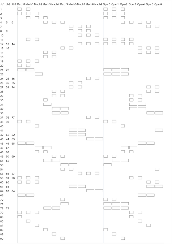
The machine and operator requirements for each job are shown in Output 3.10.1. Each row in the graph defines a resource requirement for up to three jobs that are identified in the columns Jb1–Jb3 to the left of the chart. The horizontal axis of the chart represents the resources and is split into two regions by a vertical
line. The resources to the left of the divider are the machines, Mach0–Mach9, and the resources to the right of the divider are the operators, Oper0–Oper6. For each row on the chart, a bar on the chart represents a potential requirement for the corresponding resource listed above.
Each of the jobs listed in columns Jb1–Jb3 can be processed on one of the machines in Mach0–Mach9 and requires the assistance of one of the operators in Oper0–Oper6 while being processed. An eligible resource is represented by a bar, and the length of the bar indicates the duration of
the job.
For example, row five specifies that job number 7 can be processed on machine 6, 7, or 8 and additionally requires either operator 5 or operator 6 in order to be processed. The next row indicates that jobs 8 and 9 can also be processed on the same set of machines. However, they do not require any operator assistance.
Output 3.10.1: Machine and Operator Requirements
The CLP procedure is invoked by using the following statements with FINISH=12 in the SCHEDULE statement to obtain a 12-day solution that is also known to be optimal. In order to obtain the optimal solution, it is necessary to invoke the edge-finding consistency routines, which are activated with the EDGEFINDER option in the SCHEDULE statement. The activity selection strategy is specified as DMINLS, which selects the activity with the earliest late start time. Activities with identical resource requirements are grouped together in the REQUIRES statement.
proc clp dom=[0,12] restarts=500 dpr=6 showprogress
   schedtime=schedtime_altres schedres=schedres_altres;
   schedule start=0 finish=12 actselect=dminls edgefinder;

   activity (J1-J20 J24-J30 J34-J40 J48-J50 J54-J60
             J68-J70 J74-J80 J85-J90) = (1)    /* one day jobs */
            (J21-J23 J31-J33 J41-J47 J51-J53 J61-J67
             J71-J73 J81-J84) = (2);           /* two day jobs */

   resource (M0-M9) (OP0-OP6);

   requires
      /* machine requirements */
      (J85) = (M0)
      (J1 J20 J21 J22 J38 J39 J45 J46 J65 J66) = (M0, M1)
      (J19 J2 J58 J59 J60 J78 J79 J80) = (M0, M1, M2)
      (J86) = (M1)
      (J11) = (M1, M2)
      (J3) = (M1, M2, M3)
      (J23 J40 J87) = (M2)
      (J47 J48 J67 J68) = (M2, M3)
      (J30 J31 J88) = (M3)
      (J17 J18 J51 J52 J72 J73) = (M3, M4)
      (J4 J5 J6) = (M3, M4, M5)
      (J89) = (M4)
      (J28 J29 J32 J33 J49 J50 J69) = (M4, M5)
      (J70 J71 J90) = (M5)
      (J15 J16 J53 J54) = (M5, M6)
      (J26 J27 J34 J35 J41 J42 J61 J62 J74 J75 J81 J82) = (M6, M7)
      (J7 J8 J9) = (M6, M7, M8)
      (J10 J12 J13 J14 J55 J56 J57) = (M7, M8, M9)
      (J24 J25 J36 J37 J43 J44 J63 J64 J76 J77 J83 J84) = (M8, M9)
      /* operator requirements */
      (J53 J88) = (OP0)
      (J38 J39 J49 J50 J69 J70) = (OP0, OP1)
      (J1 J2 J21 J22 J23 J3 J71 J72 J73) = (OP0, OP1, OP2)
      (J11 J12 J13 J14) = (OP0, OP1, OP2, OP3)
      (J89) = (OP1)
      (J51 J52) = (OP1, OP2)
      (J40 J90) = (OP2)
      (J47 J48 J67 J68) = (OP2, OP3)
      (J4 J5 J6) = (OP2, OP3, OP4, OP5)
      (J85) = (OP3)
      (J29 J30 J31 J32 J58 J59 J78 J79) = (OP3, OP4)
      (J86) = (OP4)
      (J45 J46 J65 J66) = (OP4, OP5)
      (J15 J16 J17) = (OP4, OP5, OP6)
      (J87) = (OP5)
      (J27 J28 J33 J34 J60 J61 J7 J74 J80 J81) = (OP5, OP6)
      (J41 J54) = (OP6);
run;
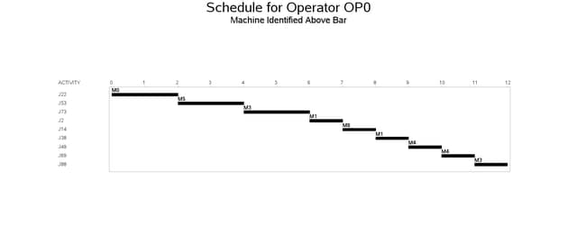
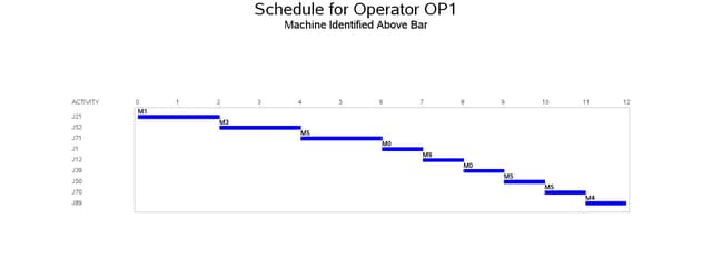
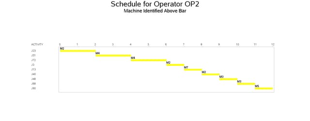
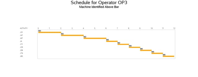
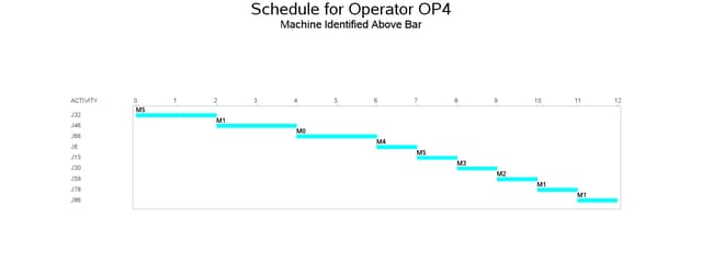
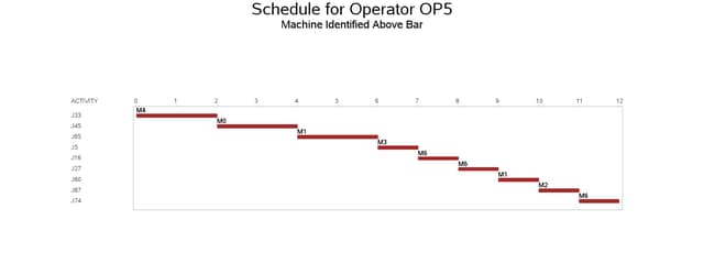
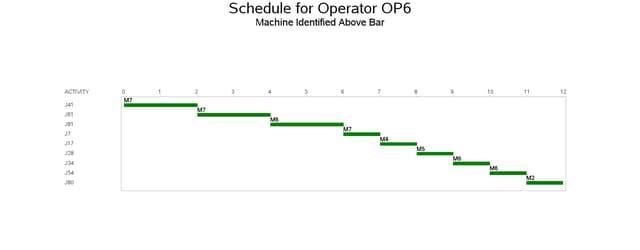
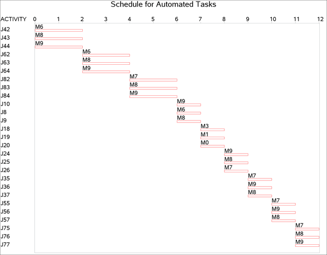
The resulting schedule is shown in a series of Gantt charts that are displayed in Output 3.10.2 and Output 3.10.3. In each of these Gantt charts, the vertical axis lists the different jobs, the horizontal bar represents the start and finish times for each of the jobs, and the text above each bar identifies the machine that the job is being processed on. Output 3.10.2 displays the schedule for the operator-assisted tasks (one for each operator), while Output 3.10.3 shows the schedule for automated tasks (that is, those tasks that do not require operator intervention).
Output 3.10.2: Operator-Assisted Jobs Schedule
Output 3.10.3: Automated Jobs Schedule
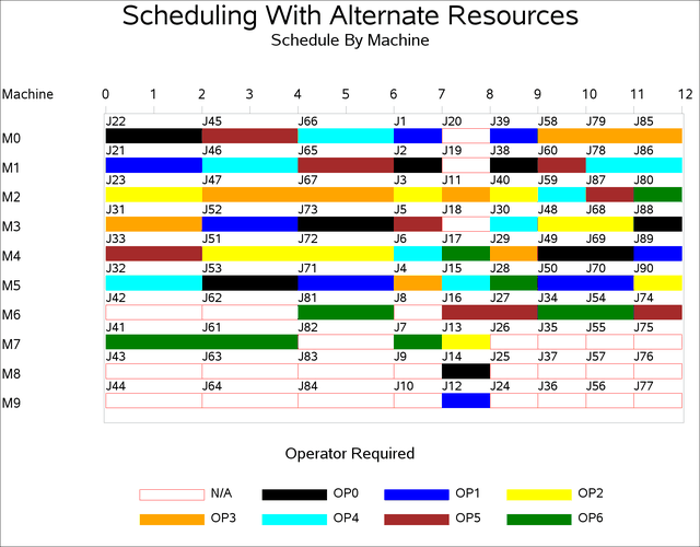
A more interesting Gantt chart is that of the resource schedule by machine, as shown in Output 3.10.4. This chart displays the schedule for each machine. Every row corresponds to a machine. Every bar on each row consists of multiple segments, and every segment represents a job that is processed on the machine. Each segment is also coded according to the operator assigned to it. The mapping of the coding is indicated in the legend. It is evident that the schedule is optimal since none of the machines or operators are idle at any time during the schedule.
Output 3.10.4: Machine Schedule