The SEVERITY Procedure
- Overview
-
Getting Started

-
Syntax
-
DetailsPredefined DistributionsCensoring and TruncationParameter Estimation MethodParameter InitializationEstimating Regression EffectsLevelization of Classification VariablesSpecification and Parameterization of Model EffectsEmpirical Distribution Function Estimation MethodsStatistics of FitDefining a Severity Distribution Model with the FCMP ProcedurePredefined Utility FunctionsScoring FunctionsCustom Objective FunctionsMultithreaded ComputationInput Data SetsOutput Data SetsDisplayed OutputODS Graphics
-
ExamplesDefining a Model for Gaussian DistributionDefining a Model for the Gaussian Distribution with a Scale ParameterDefining a Model for Mixed-Tail DistributionsEstimating Parameters Using Cramér-von Mises EstimatorFitting a Scaled Tweedie Model with RegressorsFitting Distributions to Interval-Censored DataDefining a Finite Mixture Model That Has a Scale ParameterPredicting Mean and Value-at-Risk by Using Scoring FunctionsScale Regression with Rich Regression Effects
- References
In some applications, the data available for modeling might not be exact. A commonly encountered scenario is the use of grouped data from an external agency, which for several reasons, including privacy, does not provide information about individual loss events. The losses are grouped into disjoint bins, and you know only the range and number of values in each bin. Each group is essentially interval-censored, because you know that a loss magnitude is in certain interval, but you do not know the exact magnitude. This example illustrates how you can use PROC SEVERITY to model such data.
The following DATA step generates sample grouped data for dental insurance claims, which is taken from Klugman, Panjer, and Willmot (1998):
/* Grouped dental insurance claims data
    (Klugman, Panjer, and Willmot, 1998) */
data gdental;
   input lowerbd upperbd count @@;
   datalines;
0 25 30  25 50 31  50 100 57  100 150 42  150 250 65  250 500 84
500 1000 45  1000 1500 10  1500 2500 11  2500 4000 3
;
run;
Often, when you do not know the nature of the data, it is recommended that you first explore the nature of the sample distribution by examining the nonparametric estimates of PDF and CDF. The following PROC SEVERITY step prepares the nonparametric estimates, but it does not fit any distribution because there is no DIST statement specified:
/* Prepare nonparametric estimates */
proc severity data=gdental print=all plots(histogram kernel)=all;
   loss / rc=lowerbd lc=upperbd;
   weight count;
run;
The LOSS statement specifies the left and right boundary of each group as the right-censoring and left-censoring limits, respectively.
The variable count records the number of losses in each group and is specified in the WEIGHT statement. Note that there is no response or loss
variable specified in the LOSS statement, which is allowed as long as each observation in the input data set is censored.
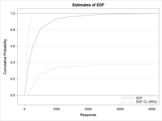
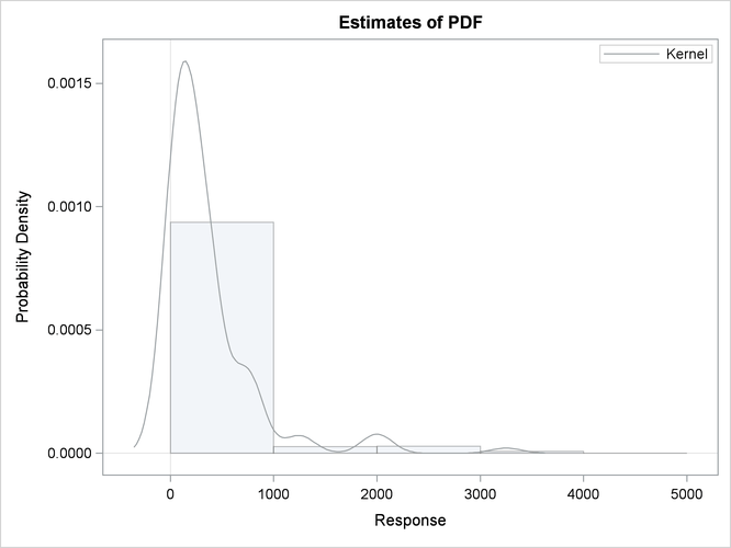
The nonparametric estimates prepared by this step are shown in Output 23.6.1. The histogram, kernel density, and EDF plots all indicate that the data is heavy-tailed. For interval-censored data, PROC
SEVERITY uses Turnbull’s algorithm to compute the EDF estimates. The plot of Turnbull’s EDF estimates is shown to be linear
between the endpoints of a censored group. The linear relationship is chosen for convenient visualization and ease of computation
of EDF-based statistics, but you should note that theoretically the behavior of Turnbull’s EDF estimates is undefined within
a group.
With the PRINT=ALL option, PROC SEVERITY prints the summary of the Turnbull EDF estimation process as shown in Output 23.6.2. It indicates that the final EDF estimates have converged and are in fact maximum likelihood (ML) estimates. If they were not ML estimates, then you could have used the ENSUREMLE option to force the algorithm to search for ML estimates.
After exploring the nature of the data, you can now fit a set of heavy-tailed distributions to this data. The following PROC
SEVERITY step fits all the predefined distributions to the data in Work.Gdental data set:
/* Fit all predefined distributions */
proc severity data=gdental print=all plots(histogram kernel)=all
              criterion=ad;
   loss / rc=lowerbd lc=upperbd;
   weight count;
   dist _predef_;
run;
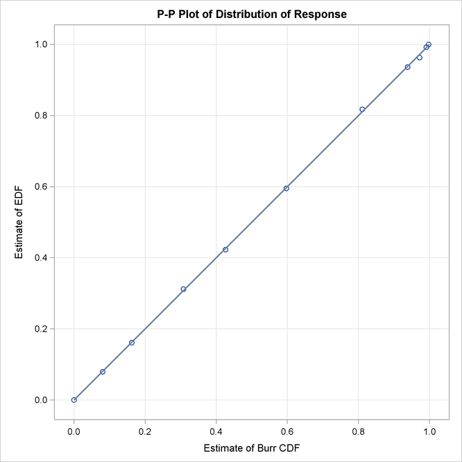
Some of the key results prepared by PROC SEVERITY are shown in Output 23.6.3 through Output 23.6.4. According to the "Model Selection" table in Output 23.6.3, all distribution models have converged. The "All Fit Statistics" table in Output 23.6.3 indicates that the generalized Pareto distribution (GPD) has the best fit for data according to a majority of the likelihood-based statistics and that the Burr distribution (BURR) has the best fit according to all the EDF-based statistics.
Output 23.6.3: Statistics of Fit for Interval-Censored Data
| All Fit Statistics | ||||||||||||||
|---|---|---|---|---|---|---|---|---|---|---|---|---|---|---|
| Distribution | -2 Log Likelihood |
AIC | AICC | BIC | KS | AD | CvM | |||||||
| Burr | 41.41112 | * | 47.41112 | 51.41112 | 48.31888 | 0.08974 | * | 0.00103 | * | 0.0000816 | * | |||
| Exp | 42.14768 | 44.14768 | * | 44.64768 | * | 44.45026 | * | 0.26412 | 0.09936 | 0.01866 | ||||
| Gamma | 41.92541 | 45.92541 | 47.63969 | 46.53058 | 0.19569 | 0.04608 | 0.00759 | |||||||
| Igauss | 42.34445 | 46.34445 | 48.05874 | 46.94962 | 0.34514 | 0.12301 | 0.02562 | |||||||
| Logn | 41.62598 | 45.62598 | 47.34027 | 46.23115 | 0.16853 | 0.01884 | 0.00333 | |||||||
| Pareto | 41.45480 | 45.45480 | 47.16908 | 46.05997 | 0.11423 | 0.00739 | 0.0009084 | |||||||
| Gpd | 41.45480 | 45.45480 | 47.16908 | 46.05997 | 0.11423 | 0.00739 | 0.0009084 | |||||||
| Weibull | 41.76272 | 45.76272 | 47.47700 | 46.36789 | 0.17238 | 0.03293 | 0.00472 | |||||||
| Note: The asterisk (*) marks the best model according to each column's criterion. | ||||||||||||||
The P-P plots of Output 23.6.4 show that both GPD and BURR have a close fit between EDF and CDF estimates, although BURR has slightly better fit, which is also indicated by the EDF-based statistics. Given that BURR is a generalization of the GPD and that the plots do not offer strong evidence in support of the more complex distribution, GPD seems like a good choice for this data.