The SEVERITY Procedure
- Overview
-
Getting Started

-
Syntax
-
DetailsPredefined DistributionsCensoring and TruncationParameter Estimation MethodParameter InitializationEstimating Regression EffectsEmpirical Distribution Function Estimation MethodsStatistics of FitDefining a Distribution Model with the FCMP ProcedurePredefined Utility FunctionsCustom Objective FunctionsMultithreaded ComputationInput Data SetsOutput Data SetsDisplayed OutputODS Graphics
-
Examples
- References
Example 23.4 Estimating Parameters Using Cramér-von Mises Estimator
PROC SEVERITY enables you to estimate model parameters by minimizing your own objective function. This example illustrates
how you can use PROC SEVERITY to implement the Cramér-von Mises estimator. Let ![]() denote the estimate of CDF at
denote the estimate of CDF at ![]() for a distribution with parameters
for a distribution with parameters ![]() , and let
, and let ![]() denote the empirical estimate of CDF (EDF) at
denote the empirical estimate of CDF (EDF) at ![]() that is computed from a sample
that is computed from a sample ![]() ,
, ![]() . Then, the Cramér-von Mises estimator of the parameters is defined as
. Then, the Cramér-von Mises estimator of the parameters is defined as
|
|
This estimator belongs to the class of minimum distance estimators. It attempts to estimate the parameters such that the squared distance between the CDF and EDF estimates is minimized.
The following PROC SEVERITY step uses the Cramér-von Mises estimator to fit four candidate distribution models, including the LOGNGPD mixed-tail distribution model that was defined in Defining a Model for Mixed-Tail Distributions. The input sample is the same as is used in that example.
options cmplib=(work.sevexmpl);

proc severity data=testmixdist obj=cvmobj print=all plots=pp;
   loss y;
   dist logngpd burr logn gpd;

   * Cramer-von Mises estimator (minimizes the distance *
   * between parametric and nonparametric estimates)    *;
   cvmobj = _cdf_(y);
   cvmobj = (cvmobj -_edf_(y))**2;
run;
The OBJ= option in the PROC SEVERITY statement specifies that the objective function cvmobj should be minimized. The programming statements compute the contribution of each observation in the input data set to the
objective function cvmobj. The use of keyword functions _CDF_ and _EDF_ makes the program applicable to all the distributions.
Some of the key results prepared by PROC SEVERITY are shown in Output 23.4.1. The “Model Selection Table” indicates that all models converged. When you specify a custom objective function, the default selection criterion is the value of the custom objective function. The “All Fit Statistics Table” indicates that LOGNGPD is the best distribution according to all the statistics of fit. Comparing the fit statistics of Output 23.4.1 with those of Output 23.3.1 indicates that the use of the Cramér-von Mises estimator has resulted in smaller values for all the EDF-based statistics of fit for all the models, which is expected from a minimum distance estimator.
Output 23.4.1: Summary of Cramér-von Mises Estimation
| Input Data Set | |
|---|---|
| Name | WORK.TESTMIXDIST |
| Label | Lognormal Body-GPD Tail Sample |
| Model Selection Table | |||
|---|---|---|---|
| Distribution | Converged | Custom Objective | Selected |
| logngpd | Yes | 0.02694 | Yes |
| Burr | Yes | 0.03325 | No |
| Logn | Yes | 0.03633 | No |
| Gpd | Yes | 2.96090 | No |
| All Fit Statistics Table | ||||||||||||||||
|---|---|---|---|---|---|---|---|---|---|---|---|---|---|---|---|---|
| Distribution | Custom | -2 Log Likelihood |
AIC | AICC | BIC | KS | AD | CvM | ||||||||
| logngpd | 0.02694 | * | 419.49635 | * | 429.49635 | * | 430.13464 | * | 442.52220 | * | 0.51332 | * | 0.21563 | * | 0.03030 | * |
| Burr | 0.03325 | 436.58823 | 442.58823 | 442.83823 | 450.40374 | 0.53084 | 0.82875 | 0.03807 | ||||||||
| Logn | 0.03633 | 491.88659 | 495.88659 | 496.01030 | 501.09693 | 0.52469 | 2.08312 | 0.04173 | ||||||||
| Gpd | 2.96090 | 560.35409 | 564.35409 | 564.47780 | 569.56443 | 2.99095 | 15.51378 | 2.97806 | ||||||||
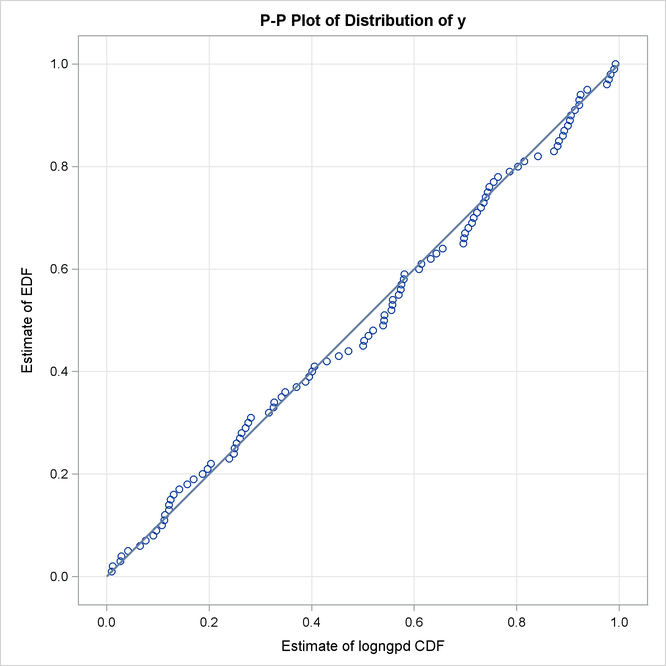
The P-P plots in Output 23.4.2 provide a visual confirmation that the CDF estimates match the EDF estimates more closely when compared to the estimates that are obtained with the maximum likelihood estimator.
Output 23.4.2: P-P Plots for LOGNGPD Model with Maximum Likelihood (Left) and Cramér-von Mises (Right) Estimators
|
|
|