The AUTOREG Procedure
- Overview
-
Getting Started

-
Syntax
-
DetailsMissing ValuesAutoregressive Error ModelAlternative Autocorrelation Correction MethodsGARCH ModelsHeteroscedasticity- and Autocorrelation-Consistent Covariance Matrix EstimatorGoodness-of-Fit Measures and Information CriteriaTestingPredicted ValuesOUT= Data SetOUTEST= Data SetPrinted OutputODS Table NamesODS Graphics
-
Examples
- References
Example 8.7 Estimation of GARCH-Type Models
This example extends Example 8.6 to include more volatility models and to perform model selection and diagnostics.
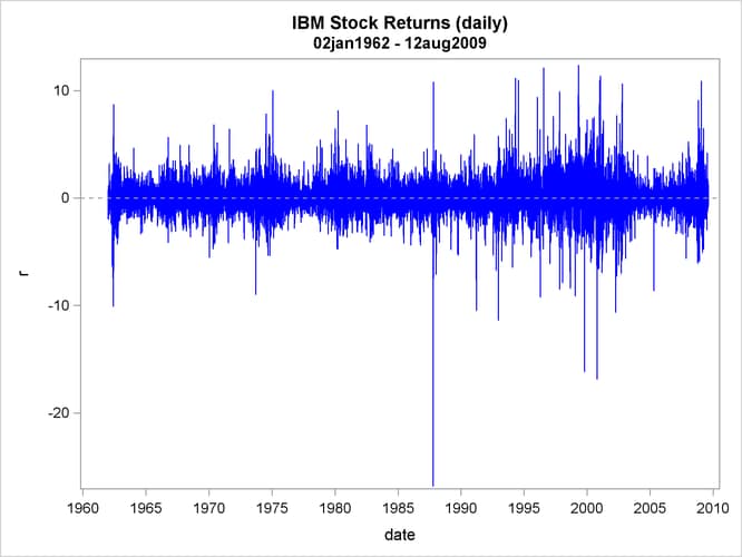
Following is the data of daily IBM stock prices for the long period from 1962 to 2009.
data ibm_long;
   infile datalines;
   format date MMDDYY10.;
   input date:MMDDYY10. price_ibm;
   r = 100*dif( log( price_ibm ) );
datalines;
01/02/1962 2.68
01/03/1962 2.7
01/04/1962 2.67
01/05/1962 2.62
01/08/1962 2.57

   ... more lines ...

08/12/2009 119.29
;
The time series of IBM returns is depicted graphically in Output 8.7.1.
Output 8.7.1: IBM Stock Returns: Daily
The following statements perform estimation of different kinds of GARCH-type models. First, ODS listing output that contains fit summary tables for each single model is captured by using an ODS OUTPUT statement with the appropriate ODS table name assigned to a new SAS data set. Along with these new data sets, another one that contains parameter estimates is created by using the OUTEST= option in AUTOREG statement.
/* Capturing ODS tables into SAS data sets */
ods output Autoreg.ar_1.FinalModel.FitSummary
           =fitsum_ar_1;
ods output Autoreg.arch_2.FinalModel.Results.FitSummary
           =fitsum_arch_2;
ods output Autoreg.garch_1_1.FinalModel.Results.FitSummary
           =fitsum_garch_1_1;
ods output Autoreg.st_garch_1_1.FinalModel.Results.FitSummary
           =fitsum_st_garch_1_1;
ods output Autoreg.ar_1_garch_1_1.FinalModel.Results.FitSummary
           =fitsum_ar_1_garch_1_1;
ods output Autoreg.igarch_1_1.FinalModel.Results.FitSummary
           =fitsum_igarch_1_1;
ods output Autoreg.garchm_1_1.FinalModel.Results.FitSummary
           =fitsum_garchm_1_1;
ods output Autoreg.egarch_1_1.FinalModel.Results.FitSummary
           =fitsum_egarch_1_1;
ods output Autoreg.qgarch_1_1.FinalModel.Results.FitSummary
           =fitsum_qgarch_1_1;
ods output Autoreg.tgarch_1_1.FinalModel.Results.FitSummary
           =fitsum_tgarch_1_1;
ods output Autoreg.pgarch_1_1.FinalModel.Results.FitSummary
           =fitsum_pgarch_1_1;

/* Estimating multiple GARCH-type models */
title "GARCH family";
proc autoreg data=ibm_long outest=garch_family;
   ar_1 :           model r = / noint nlag=1 method=ml;
   arch_2 :         model r = / noint garch=(q=2);
   garch_1_1 :      model r = / noint garch=(p=1,q=1);
   st_garch_1_1 :   model r = / noint garch=(p=1,q=1,type=stationary);
   ar_1_garch_1_1 : model r = / noint nlag=1 garch=(p=1,q=1);
   igarch_1_1 :     model r = / noint garch=(p=1,q=1,type=integ,noint);
   egarch_1_1 :     model r = / noint garch=(p=1,q=1,type=egarch);
   garchm_1_1 :     model r = / noint garch=(p=1,q=1,mean=log);
   qgarch_1_1 :     model r = / noint garch=(p=1,q=1,type=qgarch);
   tgarch_1_1 :     model r = / noint garch=(p=1,q=1,type=tgarch);
   pgarch_1_1 :     model r = / noint garch=(p=1,q=1,type=pgarch);
run;
The following statements print partial contents of the data set GARCH_FAMILY. The columns of interest are explicitly specified in the VAR statement.
/* Printing summary table of parameter estimates */
title "Parameter Estimates for Different Models";
proc print data=garch_family;
   var _MODEL_ _A_1 _AH_0 _AH_1 _AH_2
       _GH_1  _AHQ_1 _AHT_1 _AHP_1 _THETA_ _LAMBDA_ _DELTA_;
run;
These statements produce the results shown in Output 8.7.2.
Output 8.7.2: GARCH-Family Estimation Results
| Parameter Estimates for Different Models |
| Obs | _MODEL_ | _A_1 | _AH_0 | _AH_1 | _AH_2 | _GH_1 | _AHQ_1 | _AHT_1 | _AHP_1 | _THETA_ | _LAMBDA_ | _DELTA_ |
|---|---|---|---|---|---|---|---|---|---|---|---|---|
| 1 | ar_1 | 0.017112 | . | . | . | . | . | . | . | . | . | . |
| 2 | arch_2 | . | 1.60288 | 0.23235 | 0.21407 | . | . | . | . | . | . | . |
| 3 | garch_1_1 | . | 0.02730 | 0.06984 | . | 0.92294 | . | . | . | . | . | . |
| 4 | st_garch_1_1 | . | 0.02831 | 0.06913 | . | 0.92260 | . | . | . | . | . | . |
| 5 | ar_1_garch_1_1 | -0.005995 | 0.02734 | 0.06994 | . | 0.92282 | . | . | . | . | . | . |
| 6 | igarch_1_1 | . | . | 0.00000 | . | 1.00000 | . | . | . | . | . | . |
| 7 | egarch_1_1 | . | 0.01541 | 0.12882 | . | 0.98914 | . | . | . | -0.41706 | . | . |
| 8 | garchm_1_1 | . | 0.02897 | 0.07139 | . | 0.92079 | . | . | . | . | . | 0.094773 |
| 9 | qgarch_1_1 | . | 0.00120 | 0.05792 | . | 0.93458 | 0.66461 | . | . | . | . | . |
| 10 | tgarch_1_1 | . | 0.02706 | 0.02966 | . | 0.92765 | . | 0.074815 | . | . | . | . |
| 11 | pgarch_1_1 | . | 0.01623 | 0.06724 | . | 0.93952 | . | . | 0.43445 | . | 0.53625 | . |
The table shown in Output 8.7.2 is convenient for reporting the estimation result of multiple models and their comparison.
The following statements merge multiple tables that contain fit statistics for each estimated model, leaving only columns of interest, and rename them.
/* Merging ODS output tables and extracting AIC and SBC measures */
data sbc_aic;
   set fitsum_arch_2 fitsum_garch_1_1 fitsum_st_garch_1_1
       fitsum_ar_1 fitsum_ar_1_garch_1_1 fitsum_igarch_1_1
       fitsum_egarch_1_1 fitsum_garchm_1_1
       fitsum_tgarch_1_1 fitsum_pgarch_1_1 fitsum_qgarch_1_1;
   keep Model SBC AIC;
   if Label1="SBC" then do; SBC=input(cValue1,BEST12.4); end;
   if Label2="SBC" then do; SBC=input(cValue2,BEST12.4); end;
   if Label1="AIC" then do; AIC=input(cValue1,BEST12.4); end;
   if Label2="AIC" then do; AIC=input(cValue2,BEST12.4); end;
   if not (SBC=.) then output;
run;
Next, sort the models by one of the criteria, for example, by AIC:
/* Sorting data by AIC criterion */
proc sort data=sbc_aic;
   by AIC;
run;
Finally, print the sorted data set:
title "Selection Criteria for Different Models";
proc print data=sbc_aic;
   format _NUMERIC_ BEST12.4;
run;
The result is given in Output 8.7.3.
Output 8.7.3: GARCH-Family Model Selection on the Basis of AIC and SBC
| Selection Criteria for Different Models |
| Obs | Model | SBC | AIC |
|---|---|---|---|
| 1 | pgarch_1_1 | 42907.7292 | 42870.7722 |
| 2 | egarch_1_1 | 42905.9616 | 42876.3959 |
| 3 | tgarch_1_1 | 42995.4893 | 42965.9236 |
| 4 | qgarch_1_1 | 43023.106 | 42993.5404 |
| 5 | garchm_1_1 | 43158.4139 | 43128.8483 |
| 6 | garch_1_1 | 43176.5074 | 43154.3332 |
| 7 | ar_1_garch_1_1 | 43185.5226 | 43155.957 |
| 8 | st_garch_1_1 | 43178.2497 | 43156.0755 |
| 9 | arch_2 | 44605.4332 | 44583.259 |
| 10 | ar_1 | 45922.0721 | 45914.6807 |
| 11 | igarch_1_1 | 45925.5828 | 45918.1914 |
According to the smaller-is-better rule for the information criteria, the PGARCH(1,1) model is the leader by AIC while the EGARCH(1,1) is the model of choice according to SBC.
Next, check whether the power GARCH model is misspecified, especially, if dependence exists in the standardized residuals that correspond to the assumed independently and identically distributed (iid) disturbance. The following statements reestimate the power GARCH model and use the BDS test to check the independence of the standardized residuals.
proc autoreg data=ibm_long;
   model r = / noint garch=(p=1,q=1,type=pgarch) BDS=(Z=SR,D=2.0);
run;
The partial results listing of the preceding statements is given in Output 8.7.4.
Output 8.7.4: Diagnostic Checking of the PGARCH(1,1) Model
| Selection Criteria for Different Models |
| BDS Test for Independence | |||
|---|---|---|---|
| Distance | Embedding Dimension |
BDS | Pr > |BDS| |
| 2.0000 | 2 | 2.9691 | 0.0030 |
| 3 | 3.3810 | 0.0007 | |
| 4 | 3.1299 | 0.0017 | |
| 5 | 3.3805 | 0.0007 | |
| 6 | 3.3368 | 0.0008 | |
| 7 | 3.1888 | 0.0014 | |
| 8 | 2.9576 | 0.0031 | |
| 9 | 2.7386 | 0.0062 | |
| 10 | 2.5553 | 0.0106 | |
| 11 | 2.3510 | 0.0187 | |
| 12 | 2.1520 | 0.0314 | |
| 13 | 1.9373 | 0.0527 | |
| 14 | 1.7210 | 0.0852 | |
| 15 | 1.4919 | 0.1357 | |
| 16 | 1.2569 | 0.2088 | |
| 17 | 1.0647 | 0.2870 | |
| 18 | 0.9635 | 0.3353 | |
| 19 | 0.8678 | 0.3855 | |
| 20 | 0.7660 | 0.4437 | |
The results in Output 8.7.4 indicate that when embedded size is greater than 9, you fail to reject the null hypothesis of independence at 1% significance level, which is a good indicator that the PGARCH model is not misspecified.