The AUTOREG Procedure
- Overview
-
Getting Started

-
Syntax
-
DetailsMissing ValuesAutoregressive Error ModelAlternative Autocorrelation Correction MethodsGARCH ModelsHeteroscedasticity- and Autocorrelation-Consistent Covariance Matrix EstimatorGoodness-of-Fit Measures and Information CriteriaTestingPredicted ValuesOUT= Data SetOUTEST= Data SetPrinted OutputODS Table NamesODS Graphics
-
Examples
- References
Example 8.4 Missing Values
In this example, a pure autoregressive error model with no regressors is used to generate 50 values of a time series. Approximately 15% of the values are randomly chosen and set to missing. The following statements generate the data:
title  'Simulated Time Series with Roots:';
title2 ' (X-1.25)(X**4-1.25)';
title3 'With 15% Missing Values';
data ar;
   do i=1 to 550;
      e = rannor(12345);
      n = sum( e, .8*n1, .8*n4, -.64*n5 );  /* ar process  */
      y = n;
      if ranuni(12345) > .85 then y = .;    /* 15% missing */
      n5=n4; n4=n3; n3=n2; n2=n1; n1=n;     /* set lags    */
      if i>500 then output;
   end;
run;
The model is estimated using maximum likelihood, and the residuals are plotted with 99% confidence limits. The PARTIAL option prints the partial autocorrelations. The following statements fit the model:
proc autoreg data=ar partial;
   model y = / nlag=(1 4 5) method=ml;
   output out=a predicted=p residual=r ucl=u lcl=l alphacli=.01;
run;
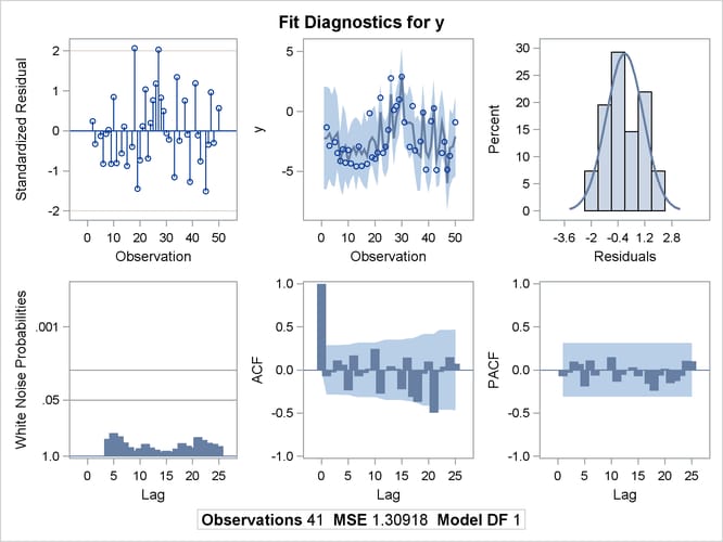
The printed output produced by the AUTOREG procedure is shown in Output 8.4.1 and Output 8.4.2. Note: the plot Output 8.4.2 can be viewed in the Autoreg.Model.FitDiagnosticPlots category by selecting →.
Output 8.4.1: Autocorrelation-Corrected Regression Results
| Simulated Time Series with Roots: |
| (X-1.25)(X**4-1.25) |
| With 15% Missing Values |
| Dependent Variable | y |
|---|
| Ordinary Least Squares Estimates | |||
|---|---|---|---|
| SSE | 182.972379 | DFE | 40 |
| MSE | 4.57431 | Root MSE | 2.13876 |
| SBC | 181.39282 | AIC | 179.679248 |
| MAE | 1.80469152 | AICC | 179.781813 |
| MAPE | 270.104379 | HQC | 180.303237 |
| Durbin-Watson | 1.3962 | Regress R-Square | 0.0000 |
| Total R-Square | 0.0000 | ||
| Parameter Estimates | |||||
|---|---|---|---|---|---|
| Variable | DF | Estimate | Standard Error |
t Value | Approx Pr > |t| |
| Intercept | 1 | -2.2387 | 0.3340 | -6.70 | <.0001 |
| Estimates of Autocorrelations | |||
|---|---|---|---|
| Lag | Covariance | Correlation | -1 9 8 7 6 5 4 3 2 1 0 1 2 3 4 5 6 7 8 9 1 |
| 0 | 4.4627 | 1.000000 | | |********************| |
| 1 | 1.4241 | 0.319109 | | |****** | |
| 2 | 1.6505 | 0.369829 | | |******* | |
| 3 | 0.6808 | 0.152551 | | |*** | |
| 4 | 2.9167 | 0.653556 | | |************* | |
| 5 | -0.3816 | -0.085519 | | **| | |
| Partial Autocorrelations | |
|---|---|
| 1 | 0.319109 |
| 4 | 0.619288 |
| 5 | -0.821179 |
| Preliminary MSE | 0.7609 |
|---|
| Estimates of Autoregressive Parameters | |||
|---|---|---|---|
| Lag | Coefficient | Standard Error |
t Value |
| 1 | -0.733182 | 0.089966 | -8.15 |
| 4 | -0.803754 | 0.071849 | -11.19 |
| 5 | 0.821179 | 0.093818 | 8.75 |
| Expected Autocorrelations | |
|---|---|
| Lag | Autocorr |
| 0 | 1.0000 |
| 1 | 0.4204 |
| 2 | 0.2480 |
| 3 | 0.3160 |
| 4 | 0.6903 |
| 5 | 0.0228 |
| Algorithm converged. |
| Maximum Likelihood Estimates | |||
|---|---|---|---|
| SSE | 48.4396756 | DFE | 37 |
| MSE | 1.30918 | Root MSE | 1.14419 |
| SBC | 146.879013 | AIC | 140.024725 |
| MAE | 0.88786192 | AICC | 141.135836 |
| MAPE | 141.377721 | HQC | 142.520679 |
| Log Likelihood | -66.012362 | Regress R-Square | 0.0000 |
| Durbin-Watson | 2.9457 | Total R-Square | 0.7353 |
| Observations | 41 | ||
| Parameter Estimates | |||||
|---|---|---|---|---|---|
| Variable | DF | Estimate | Standard Error |
t Value | Approx Pr > |t| |
| Intercept | 1 | -2.2370 | 0.5239 | -4.27 | 0.0001 |
| AR1 | 1 | -0.6201 | 0.1129 | -5.49 | <.0001 |
| AR4 | 1 | -0.7237 | 0.0914 | -7.92 | <.0001 |
| AR5 | 1 | 0.6550 | 0.1202 | 5.45 | <.0001 |
| Expected Autocorrelations | |
|---|---|
| Lag | Autocorr |
| 0 | 1.0000 |
| 1 | 0.4204 |
| 2 | 0.2423 |
| 3 | 0.2958 |
| 4 | 0.6318 |
| 5 | 0.0411 |
| Autoregressive parameters assumed given | |||||
|---|---|---|---|---|---|
| Variable | DF | Estimate | Standard Error |
t Value | Approx Pr > |t| |
| Intercept | 1 | -2.2370 | 0.5225 | -4.28 | 0.0001 |
Output 8.4.2: Diagnostic Plots
The following statements plot the residuals and confidence limits:
data reshape1;
set a;
miss = .;
if r=. then do;
miss = p;
p = .;
end;
run;
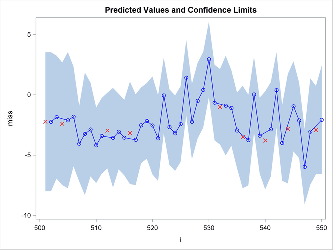
title 'Predicted Values and Confidence Limits';
proc sgplot data=reshape1 NOAUTOLEGEND;
band x=i upper=u lower=l;
scatter y=miss x=i/ MARKERATTRS =(symbol=x color=red);
series y=p x=i/markers MARKERATTRS =(color=blue) lineattrs=(color=blue);
run;
The plot of the predicted values and the upper and lower confidence limits is shown in Output 8.4.3. Note that the confidence interval is wider at the beginning of the series (when there are no past noise values to use in the forecast equation) and after missing values where, again, there is an incomplete set of past residuals.
Output 8.4.3: Plot of Predicted Values and Confidence Interval