The VARMAX Procedure
- Overview
-
Getting Started

-
Syntax
-
Details
Missing Values VARMAX Model Dynamic Simultaneous Equations Modeling Impulse Response Function Forecasting Tentative Order Selection VAR and VARX Modeling Bayesian VAR and VARX Modeling VARMA and VARMAX Modeling Model Diagnostic Checks Cointegration Vector Error Correction Modeling I(2) Model Multivariate GARCH Modeling Output Data Sets OUT= Data Set OUTEST= Data Set OUTHT= Data Set OUTSTAT= Data Set Printed Output ODS Table Names ODS Graphics Computational Issues
-
Examples
- References
| Tentative Order Selection |
Sample Cross-Covariance and Cross-Correlation Matrices
Given a stationary multivariate time series  , cross-covariance matrices are
 |
where  , and cross-correlation matrices are
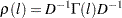 |
where  is a diagonal matrix with the standard deviations of the components of on the diagonal.
The sample cross-covariance matrix at lag  , denoted as
  , is computed as
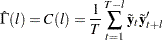 |
where  is the centered data and
  is the number of nonmissing observations. Thus,
  has
has  th element
  . The sample cross-correlation matrix at lag is computed as
 |
The following statements use the CORRY option to compute the sample cross-correlation matrices and their summary indicator plots in terms of  and
and  , where
  indicates significant positive cross-correlations,
  indicates significant negative cross-correlations, and indicates insignificant cross-correlations.
proc varmax data=simul1;
   model y1 y2 / p=1 noint lagmax=3 print=(corry)
                 printform=univariate;
run;
Figure 35.39 shows the sample cross-correlation matrices of  and
and  . As shown, the sample autocorrelation functions for each variable decay quickly, but are significant with respect to two standard errors.
| Cross Correlations of Dependent Series by Variable |
|||
|---|---|---|---|
| Variable | Lag | y1 | y2 |
| y1 | 0 | 1.00000 | 0.67041 |
| 1 | 0.83143 | 0.84330 | |
| 2 | 0.56094 | 0.81972 | |
| 3 | 0.26629 | 0.66154 | |
| y2 | 0 | 0.67041 | 1.00000 |
| 1 | 0.29707 | 0.77132 | |
| 2 | -0.00936 | 0.48658 | |
| 3 | -0.22058 | 0.22014 | |
| Schematic Representation of Cross Correlations |
||||
|---|---|---|---|---|
| Variable/Lag | 0 | 1 | 2 | 3 |
| y1 | ++ | ++ | ++ | ++ |
| y2 | ++ | ++ | .+ | -+ |
| + is > 2*std error, - is < -2*std error, . is between | ||||
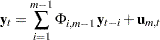
Partial Autoregressive Matrices
For each  you can define a sequence of matrices
  , which is called the partial autoregression matrices of lag
  , as the solution for to the Yule-Walker equations of order ,
 |
The sequence of the partial autoregression matrices of order has the characteristic property that if the process follows the AR( ), then
  and
and  for
for  . Hence, the matrices have the cutoff property for a VAR() model, and so they can be useful in the identification of the order of a pure VAR model.
The following statements use the PARCOEF option to compute the partial autoregression matrices:
proc varmax data=simul1;
   model y1 y2 / p=1 noint lagmax=3
                 printform=univariate
                print=(corry parcoef pcorr
                       pcancorr roots);
run;
Figure 35.40 shows that the model can be obtained by an AR order  since partial autoregression matrices are insignificant after lag 1 with respect to two standard errors. The matrix for lag 1 is the same as the Yule-Walker autoregressive matrix.
| Partial Autoregression | |||
|---|---|---|---|
| Lag | Variable | y1 | y2 |
| 1 | y1 | 1.14844 | -0.50954 |
| y2 | 0.54985 | 0.37409 | |
| 2 | y1 | -0.00724 | 0.05138 |
| y2 | 0.02409 | 0.05909 | |
| 3 | y1 | -0.02578 | 0.03885 |
| y2 | -0.03720 | 0.10149 | |
| Schematic Representation of Partial Autoregression |
|||
|---|---|---|---|
| Variable/Lag | 1 | 2 | 3 |
| y1 | +- | .. | .. |
| y2 | ++ | .. | .. |
| + is > 2*std error, - is < -2*std error, . is between | |||
Partial Correlation Matrices
Define the forward autoregression
 |
and the backward autoregression
 |
The matrices  defined by Ansley and Newbold (1979) are given by
 |
where
 |
and
 |
are the partial cross-correlation matrices at lag between the elements of  and
and  , given
  . The matrices have the cutoff property for a VAR() model, and so they can be useful in the identification of the order of a pure VAR structure.
The following statements use the PCORR option to compute the partial cross-correlation matrices:
proc varmax data=simul1;
   model y1 y2 / p=1 noint lagmax=3
                 print=(pcorr)
                 printform=univariate;
run;
The partial cross-correlation matrices in Figure 35.41 are insignificant after lag 1 with respect to two standard errors. This indicates that an AR order of can be an appropriate choice.
| Partial Cross Correlations by Variable | |||
|---|---|---|---|
| Variable | Lag | y1 | y2 |
| y1 | 1 | 0.80348 | 0.42672 |
| 2 | 0.00276 | 0.03978 | |
| 3 | -0.01091 | 0.00032 | |
| y2 | 1 | -0.30946 | 0.71906 |
| 2 | 0.04676 | 0.07045 | |
| 3 | 0.01993 | 0.10676 | |
| Schematic Representation of Partial Cross Correlations |
|||
|---|---|---|---|
| Variable/Lag | 1 | 2 | 3 |
| y1 | ++ | .. | .. |
| y2 | -+ | .. | .. |
| + is > 2*std error, - is < -2*std error, . is between | |||
Partial Canonical Correlation Matrices
The partial canonical correlations at lag between the vectors and , given , are  . The partial canonical correlations are the canonical correlations between the residual series
  and
and  , where and are defined in the previous section. Thus, the squared partial canonical correlations
  are the eigenvalues of the matrix
 |
It follows that the test statistic to test for  in the VAR model of order is approximately
 |
and has an asymptotic chi-square distribution with  degrees of freedom for .
The following statements use the PCANCORR option to compute the partial canonical correlations:
proc varmax data=simul1;
   model y1 y2 / p=1 noint lagmax=3 print=(pcancorr);
run;
Figure 35.42 shows that the partial canonical correlations  between and are {0.918, 0.773}, {0.092, 0.018}, and {0.109, 0.011} for lags
  1 to 3. After lag 1, the partial canonical correlations are insignificant with respect to the 0.05 significance level, indicating that an AR order of can be an appropriate choice.
| Partial Canonical Correlations | |||||
|---|---|---|---|---|---|
| Lag | Correlation1 | Correlation2 | DF | Chi-Square | Pr > ChiSq |
| 1 | 0.91783 | 0.77335 | 4 | 142.61 | <.0001 |
| 2 | 0.09171 | 0.01816 | 4 | 0.86 | 0.9307 |
| 3 | 0.10861 | 0.01078 | 4 | 1.16 | 0.8854 |
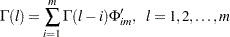
The Minimum Information Criterion (MINIC) Method
The minimum information criterion (MINIC) method can tentatively identify the orders of a VARMA(, ) process. Note that Spliid (1983), Koreisha and Pukkila (1989), and Quinn (1980) proposed this method. The first step of this method is to obtain estimates of the innovations series,
  , from the VAR(
 ), where is chosen sufficiently large. The choice of the autoregressive order, , is determined by use of a selection criterion. From the selected VAR() model, you obtain estimates of residual series
 |
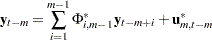
In the second step, you select the order ( ) of the VARMA model for in
  and in
 |
which minimizes a selection criterion like SBC or HQ.
The following statements use the MINIC= option to compute a table that contains the information criterion associated with various AR and MA orders:
proc varmax data=simul1;
   model y1 y2 / p=1 noint minic=(p=3 q=3);
run;
Figure 35.43 shows the output associated with the MINIC= option. The criterion takes the smallest value at AR order 1.
| Minimum Information Criterion Based on AICC | ||||
|---|---|---|---|---|
| Lag | MA 0 | MA 1 | MA 2 | MA 3 |
| AR 0 | 3.3574947 | 3.0331352 | 2.7080996 | 2.3049869 |
| AR 1 | 0.5544431 | 0.6146887 | 0.6771732 | 0.7517968 |
| AR 2 | 0.6369334 | 0.6729736 | 0.7610413 | 0.8481559 |
| AR 3 | 0.7235629 | 0.7551756 | 0.8053765 | 0.8654079 |