The VARMAX Procedure
- Overview
-
Getting Started

-
Syntax
-
Details
Missing Values VARMAX Model Dynamic Simultaneous Equations Modeling Impulse Response Function Forecasting Tentative Order Selection VAR and VARX Modeling Bayesian VAR and VARX Modeling VARMA and VARMAX Modeling Model Diagnostic Checks Cointegration Vector Error Correction Modeling I(2) Model Multivariate GARCH Modeling Output Data Sets OUT= Data Set OUTEST= Data Set OUTHT= Data Set OUTSTAT= Data Set Printed Output ODS Table Names ODS Graphics Computational Issues
-
Examples
- References
| Vector Autoregressive Process |
Let 
 denote a
  -dimensional time series vector of random variables of interest. The
  th-order VAR process is written as
 |
where the  is a vector white noise process with
 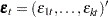 such that
  ,
,  , and
, and  for
for  ;
;  is a constant vector and
  is a
is a  matrix.
Analyzing and modeling the series jointly enables you to understand the dynamic relationships over time among the series and to improve the accuracy of forecasts for individual series by using the additional information available from the related series and their forecasts.
Example of Vector Autoregressive Model
Consider the first-order stationary bivariate vector autoregressive model
 |
The following IML procedure statements simulate a bivariate vector time series from this model to provide test data for the VARMAX procedure:
proc iml;
   sig = {1.0  0.5, 0.5 1.25};
   phi = {1.2 -0.5, 0.6 0.3};
   /* simulate the vector time series */
   call varmasim(y,phi) sigma = sig n = 100 seed = 34657;
   cn = {'y1' 'y2'};
   create simul1 from y[colname=cn];
   append from y;
quit;
The following statements plot the simulated vector time series  shown in Figure 35.1:
data simul1;
   set simul1;
   date = intnx( 'year', '01jan1900'd, _n_-1 );
   format date year4.;
run;

ods graphics on;
proc timeseries data=simul1 vectorplot=series;
   id date interval=year;
   var y1 y2;
run;
The following statements fit a VAR(1) model to the simulated data. First, you specify the input data set in the PROC VARMAX statement. Then, you use the MODEL statement to designate the dependent variables,  and
and  . To estimate a VAR model with mean zero, you specify the order of the autoregressive model with the P= option and the NOINT option. The MODEL statement fits the model to the data and prints parameter estimates and their significance. The PRINT=ESTIMATES option prints the matrix form of parameter estimates, and the PRINT=DIAGNOSE option prints various diagnostic tests. The LAGMAX=3 option is used to print the output for the residual diagnostic checks.
To output the forecasts to a data set, you specify the OUTPUT statement with the OUT= option. If you want to forecast five steps ahead, you use the LEAD=5 option. The ID statement specifies the yearly interval between observations and provides the Time column in the forecast output.
The VARMAX procedure output is shown in Figure 35.2 through Figure 35.10.
/*--- Vector Autoregressive Model ---*/

proc varmax data=simul1;
   id date interval=year;
   model y1 y2 / p=1 noint lagmax=3
                 print=(estimates diagnose);
   output out=for lead=5;
run;
The VARMAX procedure first displays descriptive statistics. The Type column specifies that the variables are dependent variables. The column N stands for the number of nonmissing observations.
Figure 35.3 shows the type and the estimation method of the fitted model for the simulated data. It also shows the AR coefficient matrix in terms of lag 1, the parameter estimates, and their significance, which can indicate how well the model fits the data.
The second table schematically represents the parameter estimates and allows for easy verification of their significance in matrix form.
In the last table, the first column gives the left-hand-side variable of the equation; the second column is the parameter name AR , which indicates the (
 )th element of the lag
  autoregressive coefficient; the last column is the regressor that corresponds to the displayed parameter.
| Type of Model | VAR(1) |
|---|---|
| Estimation Method | Least Squares Estimation |
| AR | |||
|---|---|---|---|
| Lag | Variable | y1 | y2 |
| 1 | y1 | 1.15977 | -0.51058 |
| y2 | 0.54634 | 0.38499 | |
| Schematic Representation |
|
|---|---|
| Variable/Lag | AR1 |
| y1 | +- |
| y2 | ++ |
| + is > 2*std error, - is < -2*std error, . is between, * is N/A | |
| Model Parameter Estimates | ||||||
|---|---|---|---|---|---|---|
| Equation | Parameter | Estimate | Standard Error |
t Value | Pr > |t| | Variable |
| y1 | AR1_1_1 | 1.15977 | 0.05508 | 21.06 | 0.0001 | y1(t-1) |
| AR1_1_2 | -0.51058 | 0.05898 | -8.66 | 0.0001 | y2(t-1) | |
| y2 | AR1_2_1 | 0.54634 | 0.05779 | 9.45 | 0.0001 | y1(t-1) |
| AR1_2_2 | 0.38499 | 0.06188 | 6.22 | 0.0001 | y2(t-1) | |
The fitted VAR(1) model with estimated standard errors in parentheses is given as
 |
Clearly, all parameter estimates in the coefficient matrix  are significant.
The model can also be written as two univariate regression equations.
 |
 |
 |
|||
 |
|
 |
The table in Figure 35.4 shows the innovation covariance matrix estimates and the various information criteria results. The smaller value of information criteria fits the data better when it is compared to other models. The variable names in the covariance matrix are printed for convenience;  means the innovation for , and
  means the innovation for .
Figure 35.5 shows the cross covariances of the residuals. The values of the lag zero are slightly different from Figure 35.4 due to the different degrees of freedom.
| Cross Covariances of Residuals | |||
|---|---|---|---|
| Lag | Variable | y1 | y2 |
| 0 | y1 | 1.26271 | 0.38948 |
| y2 | 0.38948 | 1.38974 | |
| 1 | y1 | 0.03121 | 0.05675 |
| y2 | -0.04646 | -0.05398 | |
| 2 | y1 | 0.08134 | 0.10599 |
| y2 | 0.03482 | -0.01549 | |
| 3 | y1 | 0.01644 | 0.11734 |
| y2 | 0.00609 | 0.11414 | |
Figure 35.6 and Figure 35.7 show tests for white noise residuals. The output shows that you cannot reject the null hypothesis that the residuals are uncorrelated.
| Cross Correlations of Residuals | |||
|---|---|---|---|
| Lag | Variable | y1 | y2 |
| 0 | y1 | 1.00000 | 0.29401 |
| y2 | 0.29401 | 1.00000 | |
| 1 | y1 | 0.02472 | 0.04284 |
| y2 | -0.03507 | -0.03884 | |
| 2 | y1 | 0.06442 | 0.08001 |
| y2 | 0.02628 | -0.01115 | |
| 3 | y1 | 0.01302 | 0.08858 |
| y2 | 0.00460 | 0.08213 | |
| Schematic Representation of Cross Correlations of Residuals |
||||
|---|---|---|---|---|
| Variable/Lag | 0 | 1 | 2 | 3 |
| y1 | ++ | .. | .. | .. |
| y2 | ++ | .. | .. | .. |
| + is > 2*std error, - is < -2*std error, . is between | ||||
| Portmanteau Test for Cross Correlations of Residuals |
|||
|---|---|---|---|
| Up To Lag | DF | Chi-Square | Pr > ChiSq |
| 2 | 4 | 1.58 | 0.8124 |
| 3 | 8 | 2.78 | 0.9473 |
The VARMAX procedure provides diagnostic checks for the univariate form of the equations. The table in Figure 35.8 describes how well each univariate equation fits the data. From two univariate regression equations in Figure 35.3, the values of  in the second column are 0.84 and 0.80 for each equation. The standard deviations in the third column are the square roots of the diagonal elements of the covariance matrix from Figure 35.4. The
  statistics are in the fourth column for hypotheses to test
  and
and  , respectively, where
  is the
  th element of the matrix . The last column shows the -values of the statistics. The results show that each univariate model is significant.
| Univariate Model ANOVA Diagnostics | ||||
|---|---|---|---|---|
| Variable | R-Square | Standard Deviation |
F Value | Pr > F |
| y1 | 0.8351 | 1.13523 | 491.25 | <.0001 |
| y2 | 0.7906 | 1.19096 | 366.29 | <.0001 |
The check for white noise residuals in terms of the univariate equation is shown in Figure 35.9. This output contains information that indicates whether the residuals are correlated and heteroscedastic. In the first table, the second column contains the Durbin-Watson test statistics to test the null hypothesis that the residuals are uncorrelated. The third and fourth columns show the Jarque-Bera normality test statistics and their -values to test the null hypothesis that the residuals have normality. The last two columns show statistics and their -values for ARCH(1) disturbances to test the null hypothesis that the residuals have equal covariances. The second table includes statistics and their -values for AR(1), AR(1,2), AR(1,2,3) and AR(1,2,3,4) models of residuals to test the null hypothesis that the residuals are uncorrelated.
| Univariate Model White Noise Diagnostics | |||||
|---|---|---|---|---|---|
| Variable | Durbin Watson |
Normality | ARCH | ||
| Chi-Square | Pr > ChiSq | F Value | Pr > F | ||
| y1 | 1.94534 | 3.56 | 0.1686 | 0.13 | 0.7199 |
| y2 | 2.06276 | 5.42 | 0.0667 | 2.10 | 0.1503 |
| Univariate Model AR Diagnostics | ||||||||
|---|---|---|---|---|---|---|---|---|
| Variable | AR1 | AR2 | AR3 | AR4 | ||||
| F Value | Pr > F | F Value | Pr > F | F Value | Pr > F | F Value | Pr > F | |
| y1 | 0.02 | 0.8980 | 0.14 | 0.8662 | 0.09 | 0.9629 | 0.82 | 0.5164 |
| y2 | 0.52 | 0.4709 | 0.41 | 0.6650 | 0.32 | 0.8136 | 0.32 | 0.8664 |
The table in Figure 35.10 gives forecasts, their prediction errors, and 95% confidence limits. See the section Forecasting for details.
| Forecasts | ||||||
|---|---|---|---|---|---|---|
| Variable | Obs | Time | Forecast | Standard Error |
95% Confidence Limits | |
| y1 | 101 | 2000 | -3.59212 | 1.13523 | -5.81713 | -1.36711 |
| 102 | 2001 | -3.09448 | 1.70915 | -6.44435 | 0.25539 | |
| 103 | 2002 | -2.17433 | 2.14472 | -6.37792 | 2.02925 | |
| 104 | 2003 | -1.11395 | 2.43166 | -5.87992 | 3.65203 | |
| 105 | 2004 | -0.14342 | 2.58740 | -5.21463 | 4.92779 | |
| y2 | 101 | 2000 | -2.09873 | 1.19096 | -4.43298 | 0.23551 |
| 102 | 2001 | -2.77050 | 1.47666 | -5.66469 | 0.12369 | |
| 103 | 2002 | -2.75724 | 1.74212 | -6.17173 | 0.65725 | |
| 104 | 2003 | -2.24943 | 2.01925 | -6.20709 | 1.70823 | |
| 105 | 2004 | -1.47460 | 2.25169 | -5.88782 | 2.93863 | |