The UCM Procedure
- Overview
-
Getting Started

-
Syntax
Functional Summary PROC UCM Statement AUTOREG Statement BLOCKSEASON Statement BY Statement CYCLE Statement DEPLAG Statement ESTIMATE Statement FORECAST Statement ID Statement IRREGULAR Statement LEVEL Statement MODEL Statement NLOPTIONS Statement OUTLIER Statement RANDOMREG Statement SEASON Statement SLOPE Statement SPLINEREG Statement SPLINESEASON Statement
-
Details
-
Examples
- References
Example 34.1 The Airline Series Revisited
The series in this example, the monthly airline passenger series, has already been discussed earlier; see the section A Seasonal Series with Linear Trend. Recall that the series consists of monthly numbers of international airline travelers (from January 1949 to December 1960). Here additional output features of the UCM procedure are illustrated, such as how to use the ESTIMATE and FORECAST statements to limit the span of the data used in parameter estimation and forecasting. The following statements fit a BSM to the logarithm of the airline passenger numbers. The disturbance variance for the slope component is held fixed at value 0; that is, the trend is locally linear with constant slope. In order to evaluate the performance of the fitted model on observed data, some of the observed data are withheld during parameter estimation and forecast computations. The observations in the last two years, years 1959 and 1960, are not used in parameter estimation, while the observations in the last year, year 1960, are not used in the forecasting computations. This is done using the BACK= option in the ESTIMATE and FORECAST statements. In addition, a panel of residual diagnostic plots is obtained using the PLOT=PANEL option in the ESTIMATE statement.
data seriesG;
   set sashelp.air;
   logair = log(air);
run;
proc ucm data = seriesG;
   id date interval = month;
   model logair;
   irregular;
   level;
   slope var = 0 noest;
   season length = 12 type=trig;
   estimate back=24 plot=panel;
   forecast back=12 lead=24 print=forecasts;
run;
The following tables display the summary of data used in estimation and forecasting (Output 34.1.1 and Output 34.1.2). These tables provide simple summary statistics for the estimation and forecast spans; they include useful information such as the beginning and ending dates of the span, the number of nonmissing values, etc.
| Variable | Type | First | Last | Nobs | Mean |
|---|---|---|---|---|---|
| logair | Dependent | JAN1949 | DEC1958 | 120 | 5.43035 |
| Variable | Type | First | Last | Nobs | Mean |
|---|---|---|---|---|---|
| logair | Dependent | JAN1949 | DEC1959 | 132 | 5.48654 |
The following tables display the fixed parameters in the model, the preliminary estimates of the free parameters, and the final estimates of the free parameters (Output 34.1.3, Output 34.1.4, and Output 34.1.5).
| Fixed Parameters in the Model | ||
|---|---|---|
| Component | Parameter | Value |
| Slope | Error Variance | 0 |
| Preliminary Estimates of the Free Parameters | ||
|---|---|---|
| Component | Parameter | Estimate |
| Irregular | Error Variance | 6.64120 |
| Level | Error Variance | 2.49045 |
| Season | Error Variance | 1.26676 |
| Final Estimates of the Free Parameters | |||||
|---|---|---|---|---|---|
| Component | Parameter | Estimate | Approx Std Error |
t Value | Approx Pr > |t| |
| Irregular | Error Variance | 0.00018686 | 0.0001212 | 1.54 | 0.1233 |
| Level | Error Variance | 0.00040314 | 0.0001566 | 2.57 | 0.0100 |
| Season | Error Variance | 0.00000350 | 1.66319E-6 | 2.10 | 0.0354 |
Two types of goodness-of-fit statistics are reported after a model is fit to the series (see Output 34.1.6 and Output 34.1.7). The first type is the likelihood-based goodness-of-fit statistics, which include the full likelihood of the data, the diffuse portion of the likelihood (see the section Details: UCM Procedure), and the information criteria. The second type of statistics is based on the raw residuals, residual = observed – predicted. If the model is nonstationary, then one-step-ahead predictions are not available for some initial observations, and the number of values used in computing these fit statistics will be different from those used in computing the likelihood-based test statistics.
| Likelihood Based Fit Statistics | |
|---|---|
| Statistic | Value |
| Full Log Likelihood | 180.63 |
| Diffuse Part of Log Likelihood | -13.93 |
| Non-Missing Observations Used | 120 |
| Estimated Parameters | 3 |
| Initialized Diffuse State Elements | 13 |
| Normalized Residual Sum of Squares | 107 |
| AIC (smaller is better) | -355.3 |
| BIC (smaller is better) | -347.2 |
| AICC (smaller is better) | -355 |
| HQIC (smaller is better) | -352 |
| CAIC (smaller is better) | -344.2 |
| Fit Statistics Based on Residuals | |
|---|---|
| Mean Squared Error | 0.00156 |
| Root Mean Squared Error | 0.03944 |
| Mean Absolute Percentage Error | 0.57677 |
| Maximum Percent Error | 2.19396 |
| R-Square | 0.98705 |
| Adjusted R-Square | 0.98680 |
| Random Walk R-Square | 0.86370 |
| Amemiya's Adjusted R-Square | 0.98630 |
| Number of non-missing residuals used for computing the fit statistics = 107 | |
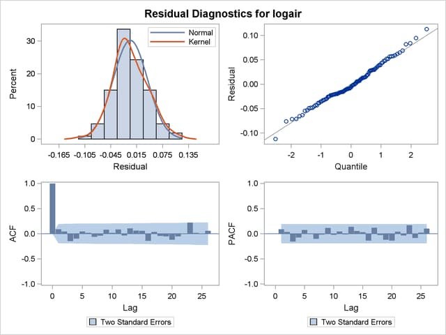
The diagnostic plots based on the one-step-ahead residuals are shown in Output 34.1.8. The residual histogram and the Q-Q plot show no reasons to question the approximate normality of the residual distribution. The remaining plots check for the whiteness of the residuals. The sample correlation plots, the autocorrelation function (ACF) and the partial autocorrelation function (PACF), also do not show any significant violations of the whiteness of the residuals. Therefore, on the whole, the model seems to fit the data well.
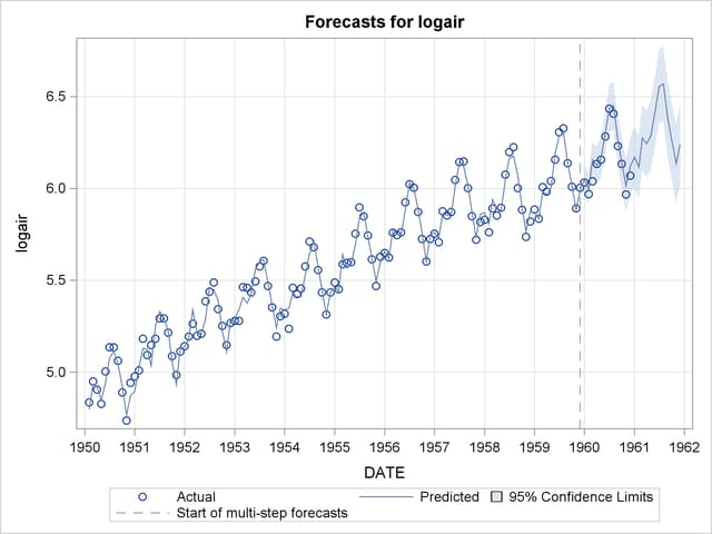
The forecasts are given in Output 34.1.9. In order to save the space,
the upper and lower confidence limit columns are dropped from the output, and only the rows corresponding to the year 1960 are shown. Recall that the actual measurements in the years 1959 and 1960 were withheld during the parameter estimation, and the ones in 1960 were not used in the forecast computations.
| Obs | date | Forecast | StdErr | logair | Residual |
|---|---|---|---|---|---|
| 133 | JAN60 | 6.050 | 0.038 | 6.033 | -0.017 |
| 134 | FEB60 | 5.996 | 0.044 | 5.969 | -0.027 |
| 135 | MAR60 | 6.156 | 0.049 | 6.038 | -0.118 |
| 136 | APR60 | 6.124 | 0.053 | 6.133 | 0.010 |
| 137 | MAY60 | 6.168 | 0.058 | 6.157 | -0.011 |
| 138 | JUN60 | 6.303 | 0.061 | 6.282 | -0.021 |
| 139 | JUL60 | 6.435 | 0.065 | 6.433 | -0.002 |
| 140 | AUG60 | 6.450 | 0.068 | 6.407 | -0.043 |
| 141 | SEP60 | 6.265 | 0.071 | 6.230 | -0.035 |
| 142 | OCT60 | 6.138 | 0.073 | 6.133 | -0.005 |
| 143 | NOV60 | 6.015 | 0.075 | 5.966 | -0.049 |
| 144 | DEC60 | 6.121 | 0.077 | 6.068 | -0.053 |
The figure Output 34.1.10 shows the forecast plot. The forecasts in the year 1960 show that the model predictions were quite good.