The UCM Procedure
- Overview
-
Getting Started

-
Syntax
Functional Summary PROC UCM Statement AUTOREG Statement BLOCKSEASON Statement BY Statement CYCLE Statement DEPLAG Statement ESTIMATE Statement FORECAST Statement ID Statement IRREGULAR Statement LEVEL Statement MODEL Statement NLOPTIONS Statement OUTLIER Statement RANDOMREG Statement SEASON Statement SLOPE Statement SPLINEREG Statement SPLINESEASON Statement
-
Details
-
Examples
- References
| The UCMs as State Space Models |
The UCMs considered in PROC UCM can be thought of as special cases of more general models, called (linear) Gaussian state space models (GSSM). A GSSM can be described as follows:
 |
 |
 |
|||
 |
|
 |
|||
 |
 |
 |
The first equation, called the observation equation, relates the response series  to a state vector
  that is usually unobserved. The second equation, called the state equation, describes the evolution of the state vector in time. The system matrices
  and
and  are of appropriate dimensions and are known, except possibly for some unknown elements that become part of the parameter vector of the model. The noise series
  consists of independent, zero-mean, Gaussian vectors with covariance matrices
  . For most of the UCMs considered here, the system matrices and , and the noise covariances , are time invariant—that is, they do not depend on time. In a few cases, however, some or all of them can depend on time. The initial state vector
  is assumed to be independent of the noise series, and its covariance matrix
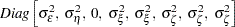
  can be partially diffuse. A random vector has a partially diffuse covariance matrix if it can be partitioned such that one part of the vector has a properly defined probability distribution, while the covariance matrix of the other part is infinite—that is, you have no prior information about this part of the vector. The covariance of the initial state is assumed to have the following form:
 |
where  and
and  are nonnegative definite, symmetric matrices and
  is a constant that is assumed to be close to
  . In the case of UCMs considered here, is always a diagonal matrix that consists of zeros and ones, and, if a particular diagonal element of is one, then the corresponding row and column in are zero.
The state space formulation of a UCM has many computational advantages. In this formulation there are convenient algorithms for estimating and forecasting the unobserved states  by using the observed series
  . These algorithms also yield the in-sample and out-of-sample forecasts and the likelihood of . The state space representation of a UCM does not need to be unique. In the representation used here, the unobserved components in the UCM often appear as elements of the state vector. This makes the elements of the state interpretable and, more important, the sample estimates and forecasts of these unobserved components are easily obtained. For additional information about the computational aspects of the state space modeling, see Durbin and Koopman (2001). Next, some notation is developed to describe the essential quantities computed during the analysis of the state space models.
Let  be the observed sample from a series that satisfies a state space model. Next, for
  , let the one-step-ahead forecasts of the series, the states, and their variances be defined as follows, using the usual notation to denote the conditional expectation and conditional variance:
 |
|
 |
|||
 |
|
 |
|||
 |
|
 |
|||
 |
|
 |
These are also called the filtered estimates of the series and the states. Similarly, for  , let the following denote the full-sample estimates of the series and the state values at time
  :
:
 |
|
 |
|||
 |
|
 |
|||
 |
|
 |
|||
 |
|
 |
If the time is in the historical period— that is, if  — then the full-sample estimates are called the smoothed estimates, and if lies in the future then they are called out-of-sample forecasts. Note that if , then
  and
and  , unless is missing.
All the filtered and smoothed estimates ( , and so on) are computed by using the Kalman filtering and smoothing (KFS) algorithm, which is an iterative process. If the initial state is diffuse, as is often the case for the UCMs, its treatment requires modification of the traditional KFS, which is called the diffuse KFS (DKFS). The details of DKFS implemented in the UCM procedure can be found in de Jong and Chu-Chun-Lin (2003). Additional information on the state space models can be found in Durbin and Koopman (2001). The likelihood formulas described in this section are taken from the latter reference.
In the case of diffuse initial condition, the effect of the improper prior distribution of manifests itself in the first few filtering iterations. During these initial filtering iterations the distribution of the filtered quantities remains diffuse; that is, during these iterations the one-step-ahead series and state forecast variances  and
and  have the following form:
 |
|
 |
|||
|
|
 |
The actual number of iterations—say,  — affected by this improper prior depends on the nature of the vectors , the number of nonzero diagonal elements of , and the pattern of missing values in the dependent series. After iterations,
  and
and  become zero and the one-step-ahead series and state forecasts have proper distributions. These first iterations constitute the initialization phase of the DKFS algorithm. The post-initialization phase of the DKFS and the traditional KFS is the same. In the state space modeling literature the pre-initialization and post-initialization phases are some times called pre-collapse and post-collapse phases of the diffuse Kalman filtering. In certain missing value patterns it is possible for to exceed the sample size; that is, the sample information can be insufficient to create a proper prior for the filtering process. In these cases, parameter estimation and forecasting is done on the basis of this improper prior, and some or all of the series and component forecasts can have infinite variances (or zero precision). The forecasts that have infinite variance are set to missing. The same situation can occur if the specified model contains components that are essentially multicollinear. In these situations no residual analysis is possible; in particular, no residuals-based goodness-of-fit statistics are produced.
The log likelihood of the sample ( ), which takes account of this diffuse initialization step, is computed by using the one-step-ahead series forecasts as follows
 |
where  is the number of diffuse elements in the initial state ,
  are the one-step-ahead residuals, and
 |
|
 |
|||
 |
|
 |
If is missing at some time , then the corresponding summand in the log likelihood expression is deleted, and the constant term is adjusted suitably. Moreover, if the initialization step does not complete—that is, if exceeds the sample size— then the value of is reduced to the number of diffuse states that are successfully initialized.
The portion of the log likelihood that corresponds to the post-initialization period is called the nondiffuse log likelihood ( ). The nondiffuse log likelihood is given by
 |
In the case of UCMs considered in PROC UCM, it often happens that the diffuse part of the likelihood,  , does not depend on the model parameters, and in these cases the maximization of nondiffuse and diffuse likelihoods is equivalent. However, in some cases, such as when the model consists of dependent lags, the diffuse part does depend on the model parameters. In these cases the maximization of the diffuse and nondiffuse likelihood can produce different parameter estimates.
In some situations it is convenient to reparameterize the nondiffuse initial state covariance as  and the state noise covariance as
  for some common scalar parameter
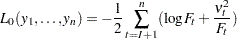
  . In this case the preceding log-likelihood expression, up to a constant, can be written as
 |
Solving analytically for the optimum, the maximum likelihood estimate of can be shown to be
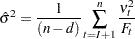 |
When this expression of is substituted back into the likelihood formula, an expression called the profile likelihood ( ) of the data is obtained:
 |
In some situations the parameter estimation is done by optimizing the profile likelihood (see the section Parameter Estimation by Profile Likelihood Optimization and the PROFILE option in the ESTIMATE statement).
In the remainder of this section the state space formulation of UCMs is further explained by using some particular UCMs as examples. The examples show that the state space formulation of the UCMs depends on the components in the model in a simple fashion; for example, the system matrix  is usually a block diagonal matrix with blocks that correspond to the components in the model. The only exception to this pattern is the UCMs that consist of the lags of dependent variable. This case is considered at the end of the section.
In what follows,  denotes a diagonal matrix with diagonal entries
  , and the transpose of a matrix is denoted as
  .
.
Locally Linear Trend Model
Recall that the dynamics of the locally linear trend model are
|
|
 |
|||
 |
|
 |
|||
 |
|
 |
Here  is the response series and
  and
and  are independent, zero-mean Gaussian disturbance sequences with variances
  , and
, and  , respectively. This model can be formulated as a state space model where the state vector
  and the state noise
  . Note that the elements of the state vector are precisely the unobserved components in the model. The system matrices
  and
and  and the noise covariance
  corresponding to this choice of state and state noise vectors can be seen to be time invariant and are given by
 |
The distribution of the initial state vector is diffuse, with 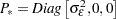 and
and 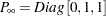 . The parameter vector
  consists of all the disturbance variances—that is,
 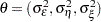 .
.
Basic Structural Model
The basic structural model (BSM) is obtained by adding a seasonal component,  , to the local level model. In order to economize on the space, the state space formulation of a BSM with a relatively short season length, season length = 4 (quarterly seasonality), is considered here. The pattern for longer season lengths such as 12 (monthly) and 52 (weekly) is easy to see.
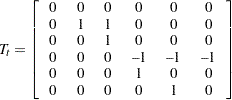
Let us first consider the dummy form of seasonality. In this case the state and state noise vectors are 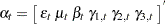 and
and 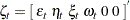 , respectively. The first three elements of the state vector are the irregular, level, and slope components, respectively. The remaining elements,
  , are lagged versions of the seasonal component .
  corresponds to lag zero—that is, the same as ,
  to lag 1 and
  to lag 2. The system matrices are
 |
and  . The distribution of the initial state vector is diffuse, with
  and
and 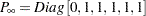 .
.
In the case of the trigonometric type of seasonality, 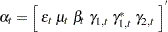 and
and 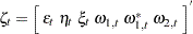 . The disturbance sequences,
  , and
, and  , are independent, zero-mean, Gaussian sequences with variance
  . The system matrices are
 |
and 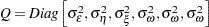 . Here
  . The distribution of the initial state vector is diffuse, with and . The parameter vector in both the cases is
 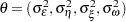 .
.
Seasons with Blocked Seasonal Values
Block seasonals are special seasonal components that impose a special block structure on the seasonal effects. Let us consider a BSM with monthly seasonality that has a quarterly block structure—that is, months within the same quarter are assumed to have identical effects except for some random perturbation. Such a seasonal component is a block seasonal with block size  equal to 3 and the number of blocks
  equal to 4. The state space structure for such a model with dummy-type seasonality is as follows: The state and state noise vectors are and , respectively. The first three elements of the state vector are the irregular, level, and slope components, respectively. The remaining elements, , are lagged versions of the seasonal component . corresponds to lag zero—that is, the same as , to lag and to lag
  . All the system matrices are time invariant, except the matrix . They can be seen to be
  , , and
 |
when is a multiple of the block size , and
 |
otherwise. Note that when is not a multiple of , the portion of the matrix corresponding to the seasonal is identity. The distribution of the initial state vector is diffuse, with and .
Similarly in the case of the trigonometric form of seasonality, and . The disturbance sequences, , and , are independent, zero-mean, Gaussian sequences with variance . 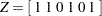 , , and
 |
when is a multiple of the block size , and
|
otherwise. As before, when is not a multiple of , the portion of the matrix corresponding to the seasonal is identity. Here . The distribution of the initial state vector is diffuse, with and . The parameter vector in both the cases is .
Cycles and Autoregression
The preceding examples have illustrated how to build a state space model corresponding to a UCM that includes components such as irregular, trend, and seasonal. There you can see that the state vector and the system matrices have a simple block structure with blocks corresponding to the components in the model. Therefore, here only a simple model consisting of a single cycle and an irregular component is considered. The state space form for more complex UCMs consisting of multiple cycles and other components can be easily deduced from this example.
Recall that a stochastic cycle  with frequency
  ,
,  , and damping coefficient
  can be modeled as
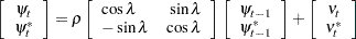 |
where  and
and  are independent, zero-mean, Gaussian disturbances with variance
  . In what follows, a state space form for a model consisting of such a stochastic cycle and an irregular component is given.
The state vector 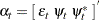 , and the state noise vector
  . The system matrices are
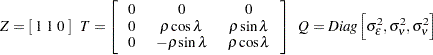 |
The distribution of the initial state vector is proper, with 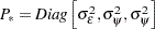 , where
  . The parameter vector
  .
.
An autoregression  can be considered as a special case of cycle with frequency equal to
  or
or  . In this case the equation for
  is not needed. Therefore, for a UCM consisting of an autoregressive component and an irregular component, the state space model simplifies to the following form.
The state vector  , and the state noise vector
  . The system matrices are
 |
The distribution of the initial state vector is proper, with 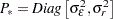 , where
  . The parameter vector
  .
.
Incorporating Predictors of Different Kinds
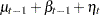
In the UCM procedure, predictors can be incorporated in a UCM in a variety of ways: simple time-invariant linear predictors are specified in the MODEL statement, predictors with time-varying coefficients can be specified in the RANDOMREG statement, and predictors that have a nonlinear relationship with the response variable can be specified in the SPLINEREG statement. As with earlier examples, how to obtain a state space form of a UCM consisting of such variety of predictors is illustrated using a simple special case. Consider a random walk trend model with predictors  , and
, and  . Let us assume that
  is a simple regressor specified in the MODEL statement,
  and
and  are random regressors with time-varying regression coefficients that are specified in the same RANDOMREG statement, and is a nonlinear regressor specified on a SPLINEREG statement. Let us further assume that the spline associated with has degree one and is based on two internal knots. As explained in the section SPLINEREG Statement, using is equivalent to using
  derived (random) regressors: say,
  . In all there are
  regressors, the first one being a simple regressor and the others being time-varying coefficient regressors. The time-varying regressors are in two groups, the first consisting of and and the other consisting of
  , and
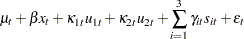
, and  . The dynamics of this model are as follows:
|
|
 |
|||
|
|
 |
|||
 |
|
 |
|||
 |
|
 |
|||
 |
|
 |
|||
 |
|
 |
|||
 |
|
 |
All the disturbances  and
and  are independent, zero-mean, Gaussian variables, where
  share a common variance parameter and
  share a common variance
  . These dynamics can be captured in the state space form by taking state
  , state disturbance
  , and the system matrices
 |
|
 |
|||
 |
|
 |
|||
 |
|
 |
Note that the regression coefficients are elements of the state vector and that the system vector is not time invariant. The distribution of the initial state vector is diffuse, with  and
and  . The parameters of this model are the disturbance variances,
  ,
, 
 and , which get estimated by maximizing the likelihood. The regression coefficients, time-invariant
  and time-varying
  and
and  , get implicitly estimated during the state estimation (smoothing).
Reporting Parameter Estimates for Random Regressors
If the random walk disturbance variance associated with a random regressor is held fixed at zero, then its coefficient is no longer time-varying. In the UCM procedure the random regressor parameter estimates are reported differently if the random walk disturbance variance associated with a random regressor is held fixed at zero. The following points explain how the parameter estimates are reported in the parameter estimates table and in the OUTEST= data set.
If the random walk disturbance variance associated with a random regressor is not held fixed, then its estimate is reported in the parameter estimates table and in the OUTEST= data set.
If more that one random regressor is specified in a RANDOMREG statement, then the first regressor in the list is used as a representative of the list while reporting the corresponding common variance parameter estimate.
If the random walk disturbance variance is held fixed at zero, then the parameter estimates table and the OUTEST= data set contain the corresponding regression parameter estimate rather than the variance parameter estimate.
Similar considerations apply in the case of the derived random regressors associated with a spline-regressor.
ARMA Irregular Component
The state space form for the irregular component that follows an ARMA(p,q) (P,Q)
(P,Q) model is described in this section. The notation for ARMA models is explained in the IRREGULAR statement. A number of alternate state space forms are possible in this case; the one given here is based on Jones (1980). With slight abuse of notation, let
  denote the effective autoregressive order and
  denote the effective moving average order of the model. Similarly, let
  be the effective autoregressive polynomial and be the effective moving average polynomial in the backshift operator with coefficients
  and
and  , obtained by multiplying the respective nonseasonal and seasonal factors. Then, a random sequence
  that follows an ARMA(p,q)(P,Q) model with a white noise sequence
  has a state space form with state vector of size
  . The system matrices, which are time invariant, are as follows:
  . The state transition matrix , in a blocked form, is given by
 |
where  if
if  and
and  is an
is an  dimensional indentity matrix. The covariance of the state disturbance matrix
  where is the variance of the white noise sequence and the vector
  contains the first values of the impulse response function—that is, the first coefficients in the expansion of the ratio
  . Since is a stationary sequence, the initial state is nondiffuse and
  . The description of
  , the covariance matrix of the initial state, is a little involved; the details are given in Jones (1980).
Models with Dependent Lags
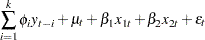
The state space form of a UCM consisting of the lags of the dependent variable is quite different from the state space forms considered so far. Let us consider an example to illustrate this situation. Consider a model that has random walk trend, two simple time-invariant regressors, and that also includes a few—say, —lags of the dependent variable. That is,
|
|
 |
|||
|
|
|
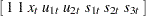
The state space form of this augmented model can be described in terms of the state space form of a model that has random walk trend with two simple time-invariant regressors. A superscript dagger ( ) has been added to distinguish the augmented model state space entities from the corresponding entities of the state space form of the random walk with predictors model. With this notation, the state vector of the augmented model
  and the new state noise vector
 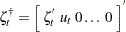 , where
  is the matrix product
  . Note that the length of the new state vector is
  . The new system matrices, in block form, are
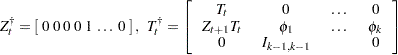 |
where  is the
  dimensional identity matrix and
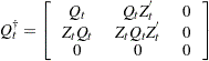 |
Note that the and matrices of the random walk with predictors model are time invariant, and in the expressions above their time indices are kept because they illustrate the pattern for more general models. The initial state vector is diffuse, with
 |
The parameters of this model are the disturbance variances and  , the lag coefficients
  , and the regression coefficients
  and
and  . As before, the regression coefficients get estimated during the state smoothing, and the other parameters are estimated by maximizing the likelihood.