The SSM Procedure (Experimental)
-
Overview

- Getting Started
-
Syntax
-
Details
The State Space Model and Notation Types of Data Organization Overview of Model Specification Syntax Likelihood, Filtering, and Smoothing Contrasting PROC SSM with Other SAS Procedures Predefined Trend Models Predefined Structural Models Covariance Parameterization Missing Values Computational Issues Displayed Output ODS Table Names OUT= Data Set
-
Examples
- References
Example 27.1 Panel Data: Two-Way Random-Effects Model
This example shows how you can use the SSM procedure to fit a two-way random-effects model to the panel data. Suppose  denotes a
  -dimensional response vector that is associated with a cross-sectional study with cross sections. The study data set contains
  measurements recorded at regular time intervals and might also contain predictor information. Here, unlike the multivariate time series setting, the values are stored in a single variable, and a separate variable called the cross-sectional variable indicates the membership of the observation to a particular cross section. Thus, for each time index
  , the information in
  takes up rows in the data set. The two-way random-effect model can be described as follows:
 |
Here the  matrix
  contains the regression variables that are associated with the
  -dimensional regression vector
  ,
,  is a -dimensional latent vector,
  is a one-dimensional latent effect,
  is a -dimensional vector with all of its entries equal to one, and
  is a -dimensional latent vector.
  is called the cross-sectional effect, is called the time effect, and
  is called the observation noise. All these latent effects are assumed to be statistically independent. In addition, it is assumed that is a zero mean, Gaussian vector with scaled identity,
  , as a covariance, is a white noise sequence with variance
  , and the observation noise is a -variate white noise sequence with covariance
  . This model can be easily formulated as an SSM that can be analyzed by using the SSM procedure as follows:
Since the random latent vector
is time-invariant, it can be specified as a state subsection with an identity as the transition matrix and zero as the state disturbance vector. Its initial condition is nondiffuse with  , a scaled identity.
 Since
affects all elements of , it must be included in the state. It can be modeled as a one-dimensional white noise state subsection. - can be modeled as observation noise, since its covariance is diagonal.
The Christenson Associates airline data, a frequently cited data set (Greene 2000), are used in this illustration. The data measure costs, prices of inputs, and utilization rates for six airlines over the time span 1970–1984. This is a cross-sectional data set with six cross sections that correspond to the six airlines; firmNumber is the cross-sectional variable and lC, the log-transformed costs, is the response variable. The following DATA step generates the data set:
data airline;
   input timePeriod firmNumber lC lQ lPF LF;
   label timePeriod  = "Time period";
   label firmNumber  = "Firm Number";
   label LF = "Load Factor (utilization index)";
   label lC = "Log transformed Costs";
   label lQ = "Log transformed Quantity";
   label lPF= "Log transformed Price of Fuel";
   year = intnx( 'year', '1jan1970'd, timePeriod-1 );
   format year year.;
datalines;
1    1    13.9471    -0.04839    11.5773    0.53449
1    2    13.2521    -0.65270    11.5502    0.49085
1    3    12.5648    -1.33781    11.6851    0.52433
1    4    11.8856    -2.44888    11.6526    0.43207

   ... more lines ...
As needed, these data are already ordered by the time index, year. For each year, there are six rows of observations—one row per airline. The following statements specify and fit a two-way random effects model to lC, the log-transformed costs. An intercept term, lQ, lPF, and LF are included as regressors.
 proc SSM data=airline;
   id year interval=year;
   parms s2c/ lower=(1.e-6);
   array firmArray{6} f1-f6;
   do j=1 to 6;
      firmArray[j] = (firmNumber=j);
   end;
   intercept = 1.0;
   state panel_state(6) T(I) cov1(I)=(s2c);
   component panel = panel_state * (firmArray);
   state t_noise(1) type=wn cov(D);
   component teffect = t_noise[1];
   irregular wn ;
   model lC = intercept lQ lPF LF panel teffect wn;
   eval trendPlusReg = intercept + lQ + lPF + LF +
     panel + teffect;
   forecast out=for;
run;
The ID statement specifies year as an ID variable with yearly frequency. The PARMS statement defines s2c, a parameter that is restricted to be positive. s2c is used later as the variance parameter for the panel effect. An array, firmArray, is defined, which is used later to pick the correct element of in a COMPONENT statement. A constant column, intercept, is defined to be used later as an intercept term. The state subsection panel_state corresponds to , and the component panel extracts the proper element of by using firmArray. The component teffect corresponds to , and wn specifies the observation noise . Finally the MODEL statement defines the model. A state linear combination, rendPlusReg, defined by the EVAL statement, is a sum of all effects in the model except the observation noise. An output data set, for, is specified to output all the estimated components. Some of the tables produced by running these statements are shown in Output 27.1.1 through Output 27.1.6.
The model summary, shown in Output 27.1.1, shows that the model is defined by one MODEL statement, the dimension of the underlying state vector is 7 (since is six-dimensional and is one-dimensional), the diffuse dimension is 4 (because of the four predictors in the model), and there are three parameters to be estimated.
| Model Summary | |
|---|---|
| Model Property | Value |
| Number of Model Equations | 1 |
| State Dimension | 7 |
| Dimension of the Diffuse Initial Condition | 4 |
| Number of Parameters | 3 |
| ID Variable Information | ||||
|---|---|---|---|---|
| Name | Start | End | MaxDelta | Type |
| year | 1970 | 1984 | 1.00 | Regular with replication |
| Likelihood Based Fit Statistics | |
|---|---|
| Statistic | Value |
| Non-Missing Response Values Used | 90 |
| Estimated Parameters | 3 |
| Initialized Diffuse State Elements | 4 |
| Normalized Residual Sum of Squares | 86 |
| Full Log Likelihood | 109.15 |
| AIC (smaller is better) | -212.3 |
| BIC (smaller is better) | -204.9 |
| AICC (smaller is better) | -212 |
| HQIC (smaller is better) | -209.3 |
| CAIC (smaller is better) | -201.9 |
| Estimates of the Regression Parameters | |||||
|---|---|---|---|---|---|
| Response Variable | Regression Variable | Estimate | Approx Std Error |
t Value | Approx Pr > |t| |
| lC | intercept | 9.36918 | 0.24003 | 39.03 | <.0001 |
| lC | lQ | 0.86746 | 0.02510 | 34.56 | <.0001 |
| lC | lPF | 0.43596 | 0.01700 | 25.64 | <.0001 |
| lC | LF | -0.98529 | 0.22369 | -4.40 | <.0001 |
 , the panel effect variance.
 | Maximum Likelihood Estimates of the Parameters Specified in the PARMS Statement |
||
|---|---|---|
| Parameter | Estimate | Approx Std Error |
| s2c | 0.01516 | 0.0097921 |
. | Maximum Likelihood Estimates of the Unknown System Parameters (Parameters Not Specified in the PARMS Statement) | ||||
|---|---|---|---|---|
| Component | Type | Parameter | Estimate | Approx Std Error |
| t_noise | Disturbance Covariance | Cov[1, 1] | 0.00107 | 0.0006450 |
| wn | Irregular | Variance | 0.00274 | 0.0004721 |
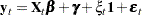
Very often the main goal of a panel study is to estimate the regression effects, having taken into account the panel-specific intercepts (). However, you might also be interested in other issues. For example, the scatter plot in Output 27.1.7 shows the smoothed estimates of between 1970 and 1984, which can be thought of as shocks to the overall airline industry during this span. This plot is produced by using smoothed_teffect, the smoothed estimate of the teffect component in the model.
  proc sgplot data=for;
     title "Yearly Disturbances to the Airline Industry";
     scatter x=year y=smoothed_teffect;
     refline 0;
 run;
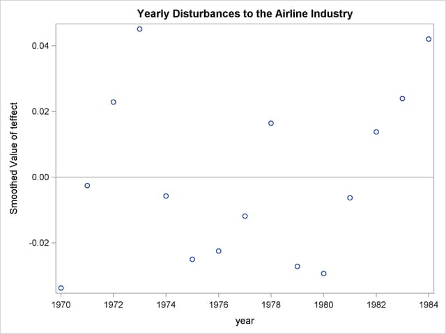
Similarly, you might wish to study the company-specific patterns implied by the fitted model. This can be done by using the smoothed estimate of trendPlusReg, a component defined by the EVAL statement in the program. The output data set, for, contains this estimate and contains its 95%confidence limits. However, firmNumber, the input data set variable that contains the company number, is not output to for. The following DATA step merges for with the input data set airline:
data for;
   merge for airline;
   by year;
run;
The following statements produce a panel of airline-specific trends. It is shown in Output 27.1.8.
  proc sgpanel data=for noautolegend;
   title 'Airline-specific Trends';
      panelby firmNumber / columns=3;
      band x=year lower=smoothed_lower_trendplusReg
         upper=smoothed_upper_trendplusReg;
      scatter x=year y=lC;
      series  x=year y= smoothed_trendplusReg;
  run;
Note: This procedure is experimental.