The SSM Procedure (Experimental)

Predefined Structural Models

A set of predefined models is available in the SSM procedure for models called structural models in the time series literature. These predefined models can be used to model trend, seasonal, and cyclical patterns in the univariate and multivariate time series. For the most part, the multivariate models are straightforward generalizations of the corresponding univariate models—for example, the multivariate random walk trend described later in this section generalizes the univariate random walk trend described in the section Random Walk Trend. All of these models, with the exception of the continuous-time cycle model, are applicable only to the regular data type. The continuous-time cycle model is applicable to all the data types; however, it is available for the univariate case only.

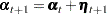
To specify these models, you must first use the STATE statement with the correct TYPE= option. When you specify the TYPE=option, you do not need to specify other options of the STATE statement (for example, the T option, the COV1 option, and the A1 option). However, you must specify the COV option, which describes the covariance of the disturbance term that drives the state equation. Throughout this section, the symmetric matrix specified by using the COV option is denoted by $\text{[math]}$ . For TYPE= LL, an additional matrix, specified by using the SLOPECOV suboption, also plays a role. It is denoted by $\text{[math]}$ . Subsequently you must specify one or more COMPONENT statements to define the (univariate) components based on this state subsection for their inclusion in the MODEL statement. These univariate components exhibit interesting behavior based on the structure of $\text{[math]}$ (and $\text{[math]}$ , whenever applicable)—for example, imposing rank restrictions on $\text{[math]}$ in the multivariate random walk results in these univariate trends moving together. For additional information about these models, see Harvey (1989).

The following example summarizes the steps needed to define a multivariate structural model by using a sequence of STATE and COMPONENT statements. For a full example, see the section Getting Started: SSM Procedure. Suppose that a three-dimensional time series is being studied with response variables y1, y2, and y3. Suppose you want to specify the three-variate structural model

$\text{[math]}$

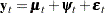where 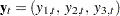$\text{[math]}$ denotes the response series, and $\text{[math]}$ , $\text{[math]}$ , and $\text{[math]}$ denote the three-variate components, trend, cycle, and white noise, respectively. The three components of $\text{[math]}$ , the observation noise in the model, are not assumed to be independent. Therefore, you cannot specify them by using three IRREGULAR statements; you must include them in the state specification. The following (incomplete) statements show how to specify this model:

     state whiteNoise(3)  type=wn ...;
     component wn1 =  whiteNoise[1];
     component wn2 =  whiteNoise[2];
     component wn3 =  whiteNoise[3];
     
     state randomWalk(3)  type=rw ...;
     component rw1 =  randomWalk[1];
     component rw2 =  randomWalk[2];
     component rw3 =  randomWalk[3];
     
     state cycleState(3)  type=cycle ...;
     component c1 = cycleState[1];
     component c2 = cycleState[2];
     component c3 = cycleState[3];
     
     model y1 = rw1 c1 wn1;
     model y2 = rw2 c2 wn2;
     model y3 = rw3 c3 wn3;

The first STATE statement defines whiteNoise, a state subsection needed for defining a three-dimensional white noise component. In turn, whiteNoise is used to define the three univariate white noise components: wn1, wn2, and wn3. The components wn1, wn2, and wn3 are correlated—their correlation structure is controlled by the covariance specification of whiteNoise. The second set of STATE and COMPONENT statements result in three correlated random walk trend components: rw1, rw2, and rw3. Finally, the last set of STATE and COMPONENT statements result in three correlated cycle components: c1, c2, and c3. In the end, the desired multivariate model is defined by including these (univariate) components in the appropriate MODEL statements.

In the preceding example, it is important to note the relationship between the dimension, denoted by dim throughout this section, specified in the STATE statement and the actual dimension of the resulting state subsection. Note that the three state subsections, whiteNoise, randomWalk, and cycleState, are defined by using the same dim specification: 3. However, the actual dimensions of these state subsections depend on their type; they do not need to equal this specified dimension. Here, whiteNoise and randomWalk do have the same size, 3, as the specified dim. However, the size of cycleState, which is of TYPE=CYCLE, is $\text{[math]}$ . Another important point to note: no matter what the underlying size of the state subsection, the desired univariate components were obtained by using an identical specification scheme in the COMPONENT statement. This happens because the component specification style based on the element operator—[]—in the COMPONENT statement behaves differently when the TYPE= option is used to define the state subsection (see the section Multivariate Season for an illustration).

The system matrices for all these models are time-invariant, with the exception of the continuous-time cycle model. In this section, $\text{[math]}$ denotes the subsection of the overall model state $\text{[math]}$ , and $\text{[math]}$ , $\text{[math]}$ , and $\text{[math]}$ denote the corresponding blocks of the larger system matrices.

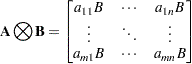
For the multivariate cycle system matrices described in the section Multivariate Cycle, the Kronecker product notation is useful: if $\text{[math]}$ is an $\text{[math]}$ matrix and $\text{[math]}$ is a $\text{[math]}$ matrix, then the Kronecker product $\text{[math]}$ is an $\text{[math]}$ block matrix:

$\text{[math]}$

Multivariate White Noise

The STATE statement option TYPE=WN specifies white noise of dimension dim—that is, a sequence of zero mean, independent, Gaussian vectors with covariance $\text{[math]}$ . The specification of the associated system matrices is trivial: $\text{[math]}$ is zero, $\text{[math]}$ , and the initial condition is nondiffuse ( $\text{[math]}$ and $\text{[math]}$ ).

Multivariate white noise is needed to specify the observation equation noise term for the multivariate models for the time series data. Since the state space formulation for the SSM procedure requires the observation equation noise vector to have the diagonal form, you need to include the noise vector in the state. The noise term for the $\text{[math]}$ th response variable is defined by a component that simply picks the $\text{[math]}$ th element of this multivariate white noise. For example, the component wn_i defined as follows can be used as a noise term in the MODEL statement of the $\text{[math]}$ th response variable:

     state white(dim) type=wn ...;
     component wn_i = white[i];

Multivariate Random Walk Trend

The STATE statement option TYPE=RW specifies a dim-dimensional random walk

$\text{[math]}$

where $\text{[math]}$ is a sequence of zero mean, independent, Gaussian vectors with covariance $\text{[math]}$ . The specification of the associated system matrices is trivial: $\text{[math]}$ is a dim-dimensional identity matrix, $\text{[math]}$ , $\text{[math]}$ , and the initial condition is fully diffuse ( $\text{[math]}$ and $\text{[math]}$ ).

The multivariate random walk is a useful trend model for multivariate time series data. The trend term for the $\text{[math]}$ th response variable is defined by a component that simply picks the $\text{[math]}$ th ( $\text{[math]}$ ) element of $\text{[math]}$ . For example, the component rw_i defined as follows can be used as a trend term in the MODEL statement of the $\text{[math]}$ th response variable:

     state randomWalk(dim) type=rw ...;
     component rw_i = randomWalk[i];

Multivariate Local Linear Trend

The STATE statement option TYPE=LL specifies a (2*dim)-dimensional $\text{[math]}$ , needed for defining a dim-dimensional local linear trend. The first dim elements of $\text{[math]}$ correspond to the needed multivariate trend, and the subsequent dim elements are needed to capture the slope vector of this trend. $\text{[math]}$ can be defined as

$\text{[math]}$

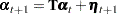where $\text{[math]}$ is a sequence of zero mean, independent, Gaussian vectors with covariance $\text{[math]}$ and $\text{[math]}$ is a 2*dim-dimensional block matrix 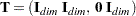$\text{[math]}$ . The initial condition is fully diffuse ( $\text{[math]}$ and $\text{[math]}$ ). This is a multivariate generalization of the univariate local linear trend.

The multivariate local linear trend is a useful trend model for multivariate time series data. The trend term for the $\text{[math]}$ th response variable is defined by a component that simply picks the $\text{[math]}$ th element ( $\text{[math]}$ ) of $\text{[math]}$ . For example, the component ll_i defined as follows can be used as a trend term in the MODEL statement of the $\text{[math]}$ th response variable:

     state localLin(dim) type=ll(slopecov..) ...;
     component ll_i = localLin[i];

Multivariate Cycle

The STATE statement option TYPE=CYCLE specifies a (2*dim)-dimensional $\text{[math]}$ , needed for defining a dim-dimensional cycle. As in the LL case, the first dim elements of $\text{[math]}$ correspond to the needed dim-dimensional cycle, and the remaining dim elements contain some auxiliary quantities. The cycle model defined in this subsection requires a regular data type—that is, the CT option is not included. Let $\text{[math]}$ denote the damping factor, and $\text{[math]}$ period be the frequency associated with the cycle. The admissible parameter ranges are $\text{[math]}$ and period $\text{[math]}$ , which implies that $\text{[math]}$ . 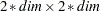Let $\text{[math]}$ , a $\text{[math]}$ matrix, and let $\text{[math]}$ , a $\text{[math]}$ matrix. With this notation, the transition equation associated with $\text{[math]}$ is

$\text{[math]}$

where $\text{[math]}$ is a sequence of zero mean, independent, $\text{[math]}$ -dimensional Gaussian vectors with covariance $\text{[math]}$ . If $\text{[math]}$ , the initial condition is fully diffuse ( $\text{[math]}$ and $\text{[math]}$ ). Otherwise, it is nondiffuse: 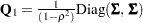$\text{[math]}$ and $\text{[math]}$ .

The multivariate cycle is useful for capturing periodic behavior for multivariate time series data. The cycle term for the $\text{[math]}$ th response variable is defined by a component that simply picks the $\text{[math]}$ th element of $\text{[math]}$ . For example, the component cycle_i defined as follows can be used as a cycle term in the MODEL statement of the $\text{[math]}$ th response variable:

     state cycleState(dim) type=cycle  ...;
     component cycle_i = cycleState[i];

Multivariate Season

The STATE statement option TYPE=SEASON(LENGTH=s) specifies a ((s–1)*dim)-dimensional $\text{[math]}$ , needed for defining a dim-dimensional trigonometric season component with season length s. A (multivariate) trigonometric season component, $\text{[math]}$ , is a sum of (multivariate) cycles of different frequencies,

$\text{[math]}$

where the constituent cycles $\text{[math]}$ , called harmonics, have frequencies $\text{[math]}$ s. All the harmonics are assumed to be statistically independent, have the same damping factor $\text{[math]}$ , and are governed by the disturbances with the same covariance matrix $\text{[math]}$ . The number of harmonics, $\text{[math]}$ , equals $\text{[math]}$ if $\text{[math]}$ is even and $\text{[math]}$ if it is odd. This means that specifying TYPE=SEASON(LENGTH=s) is equivalent to specifying $\text{[math]}$ cycle specifications with correct frequencies, damping factor $\text{[math]}$ , and the COV option restricted to the same covariance $\text{[math]}$ . The resulting $\text{[math]}$ is necessarily ((s–1)*dim)-dimensional. When the season length $\text{[math]}$ is even, the last harmonic cycle, $\text{[math]}$ , has frequency $\text{[math]}$ and requires special attention. It is of dimension dim rather than 2*dim because its underlying state equation simplifies to a dim-variate autoregression with autoregression coefficient $\text{[math]}$ . As a result of this discussion, it is clear that the system matrices $\text{[math]}$ and $\text{[math]}$ associated with the ((s–1)*dim)-dimensional $\text{[math]}$ are block-diagonal with the blocks corresponding to the harmonics. The initial condition is fully diffuse.

For all the models discussed so far, the first dim elements of $\text{[math]}$ provided the needed (multivariate) component. This is not the case for the (multivariate) season component. Extracting the $\text{[math]}$ th seasonal component from $\text{[math]}$ requires accumulating the contributions from the $\text{[math]}$ harmonics associated with this $\text{[math]}$ th seasonal, which are not organized contiguously in $\text{[math]}$ . For example, suppose that dim is 2 and the season length s is 4. In this case $\text{[math]}$ is 2, and the bivariate seasonal component is a sum of two independent bivariate cycles, $\text{[math]}$ and $\text{[math]}$ . The cycle $\text{[math]}$ has frequency $\text{[math]}$ and its underlying state, say $\text{[math]}$ , has dimension $\text{[math]}$ . The last harmonic, $\text{[math]}$ , has frequency $\text{[math]}$ , and therefore its underlying state, say $\text{[math]}$ , has dimension 2. The combined state $\text{[math]}$ has dimension $\text{[math]}$ . In order to extract the first bivariate seasonal component, you must extract the first components of bivariate cycles $\text{[math]}$ and $\text{[math]}$ , which in turn implies the first elements of $\text{[math]}$ and $\text{[math]}$ , respectively. Thus, obtaining the first bivariate seasonal component requires extracting the first and the fifth elements of the combined state $\text{[math]}$ . Similarly, obtaining the second bivariate seasonal component requires extracting the second and the sixth elements of the combined state $\text{[math]}$ . All this can be summarized by the dot product expressions

	$\text{[math]}$	$\text{[math]}$	$\text{[math]}$
	$\text{[math]}$	$\text{[math]}$	$\text{[math]}$

where $\text{[math]}$ and $\text{[math]}$ denote the first and second components, respectively, of the bivariate seasonal component. Note that $\text{[math]}$ and $\text{[math]}$ are univariate seasonal components, each of season length $\text{[math]}$ , in their own right. They are correlated components; their correlation structure depends on $\text{[math]}$ .

Obtaining the desired components of the multivariate seasonal component is made easy by a special syntax convention of the COMPONENT statement. Continuing with the previous example, the following examples illustrate two equivalent ways of obtaining $\text{[math]}$ and $\text{[math]}$ . The first set of statements explicitly specify the linear combinations needed for defining $\text{[math]}$ and $\text{[math]}$ :

     state seasonState(2) type=season(length=4)  ...;
     component s_1 =( 1  0  0  0  1  0 ) * seasonState;
     component s_2 =( 0  1  0  0  0  1 ) * seasonState;

The following simpler specification achieves the same result:

     state seasonState(2) type=season(length=4)  ...;
     component s_1 = seasonState[1];
     component s_2 = seasonState[2];

In the latter specification, the meaning of the element operator [] changes if the state in question is defined by using the TYPE= option.

Continuous-Time Cycle

The STATE statement option TYPE=CYCLE(CT) specifies a two-dimensional $\text{[math]}$ , needed for defining a univariate continuous time cycle. In this case the dimension, dim, used in the STATE statement must be 1. In particular, $\text{[math]}$ becomes one-dimensional, which is denoted by $\text{[math]}$ . This cycle can be used for any data type. As before, the parameters of the cycle are a damping factor $\text{[math]}$ , $\text{[math]}$ , and period $\text{[math]}$ . Unlike in the discrete-time cycle described in the section Multivariate Cycle, the period is not required to be larger than 2. Let $\text{[math]}$ and let $\text{[math]}$ denote the difference between successive time points. In this case, the system matrices $\text{[math]}$ and $\text{[math]}$ that govern $\text{[math]}$ depend on $\text{[math]}$ . They are:

$\text{[math]}$	$\text{[math]}$	$\text{[math]}$
$\text{[math]}$	$\text{[math]}$	$\text{[math]}$
$\text{[math]}$	$\text{[math]}$	$\text{[math]}$

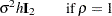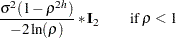
If $\text{[math]}$ , the initial condition is nondiffuse: $\text{[math]}$ . For $\text{[math]}$ , the initial condition is fully diffuse.

The first element of $\text{[math]}$ corresponds to the needed cycle, and the second element is an auxiliary quantity. You can define a cycle term based on this state as follows:

     state cycleState(1) type=cycle(CT)  ...;
     component cycle = cycleState[1];

Note that the CT option must be included in the use of TYPE=CYCLE.

Note: This procedure is experimental.