The SSM Procedure (Experimental)

Getting Started: SSM Procedure

This example illustrates how you can use the SSM procedure to analyze a bivariate time series. The following data set contains two variables, f_KSI and r_KSI, which are measured quarterly, starting on the first quarter of 1969. f_KSI represents the quarterly average of the log of the monthly totals of the front-seat passengers killed or seriously injured during the car accidents, and r_KSI represents a similar number for the rear-seat passengers. The data set has been extended at the end with eight missing values, which represent four quarters, to cause the SSM procedure to produce model forecasts for this span.

data seatBelt; 
input f_KSI r_KSI @@;  
label f_KSI = "Front Seat Passengers Injured--log scale";
label r_KSI = "Rear Seat Passengers Injured--log scale";
date = intnx( 'quarter', '1jan1969'd, _n_-1 );  
format date YYQS.;
datalines;
    6.72417 5.64654  6.81728 6.06123  6.92382 6.18190
    6.92375 6.07763  6.84975 5.78544  6.81836 6.04644
    7.00942 6.30167  7.09329 6.14476  6.78554 5.78212
    6.86323 6.09520  6.99369 6.29507  6.98344 6.06194
    6.81499 5.81249  6.92997 6.10534  6.96356 6.21298
    7.02296 6.15261  6.76466 5.77967  6.95563 6.18993
    7.02016 6.40524  6.87849 6.06308  6.55966 5.66084
    6.73627 6.02395  6.91553 6.25736  6.83576 6.03535
    6.52075 5.76028  6.59860 5.91208  6.70597 6.08029
    6.75110 5.98833  6.53117 5.67676  6.52718 5.90572
    6.65963 6.01003  6.76869 5.93226  6.44483 5.55616
    6.62063 5.82533  6.72938 6.04531  6.82182 5.98277
    6.64134 5.76540  6.66762 5.91378  6.83524 6.13387
    6.81594 5.97907  6.60761 5.66838  6.62985 5.88151
    6.76963 6.06895  6.79927 6.01991  6.52728 5.69113
    6.60666 5.92841  6.72242 6.03111  6.76228 5.93898
    6.54290 5.72538  6.62469 5.92028  6.73415 6.11880
    6.74094 5.98009  6.46418 5.63517  6.61537 5.96040
    6.76185 6.15613  6.79546 6.04152  6.21529 5.70139
    6.27565 5.92508  6.40771 6.13903  6.37293 5.96883
    6.16445 5.77021  6.31242 6.05267  6.44414 6.15806
    6.53678 6.13404 . . . . . . . .
run;

These data have been analyzed in Durbin and Koopman (2001, chap. 9, sec. 3). The analysis presented here is similar but not the same. In order to simplify the illustration, the monthly data have been converted to quarterly data, and two predictors (the number of kilometers traveled and the real price of petrol) are excluded from the analysis. You can also use PROC SSM to carry out the more elaborate analysis in Durbin and Koopman (2001).

One of the original reasons for studying these data was to assess the effect on f_KSI of the enactment of a seat-belt law in February 1983 that compelled the front seat passengers to wear seat belts. A simple graphical inspection of the data (not shown here) reveals that f_KSI and r_KSI do not show a pronounced upward or downward trend but do show seasonal variation, and that these two series seem to move together. Additional inspection also shows that the seasonal effect is relatively stable throughout the data span. These considerations suggest the following model for $\text{[math]}$ = (f_KSI, r_KSI):

$\text{[math]}$

All the terms on the right-hand side of this equation are assumed to be statistically independent. These terms are as follows:

The predictor $\text{[math]}$ (defined as Q1_83_Shift later in the program) denotes a variable that is 0 before the first quarter of 1983, and 1 thereafter. $\text{[math]}$ is supposed to affect only f_KSI (the first element of $\text{[math]}$ ); it represents the enactment of the seat-belt law of 1983.
$\text{[math]}$ denotes a bivariate random walk. It is supposed to capture the slowly changing level of the vector $\text{[math]}$ . In order to capture the fact that f_KSI and r_KSI move together (that is, they are co-integrated), the covariance of the disturbance term of this random walk is assumed to be of lower than full rank.
$\text{[math]}$ denotes a bivariate trigonometric seasonal term. In this model it is taken to be fixed (that is, the seasonal effects do not change over time).
$\text{[math]}$ denotes a bivariate white noise term, which captures the residual variation that is unexplained by the other terms in the model.

The preceding model is an example of a (bivariate) basic structural model (BSM). You can formulate this model as a state space model

$\text{[math]}$	$\text{[math]}$	$\text{[math]}$
$\text{[math]}$	$\text{[math]}$	$\text{[math]}$
$\text{[math]}$	$\text{[math]}$	$\text{[math]}$

for some suitable matrices $\text{[math]}$ , and $\text{[math]}$ , unobserved state vectors $\text{[math]}$ , and disturbance vectors $\text{[math]}$ . The initial state vector $\text{[math]}$ is partially diffuse: it is the sum of a mean-zero Gaussian vector $\text{[math]}$ and a term $\text{[math]}$ that represents the contribution from a diffuse vector $\text{[math]}$ (a diffuse vector is a Gaussian vector with infinite covariance). See the section The State Space Model and Notation for more information about the state space model notation. In fact, each of the terms $\text{[math]}$ , $\text{[math]}$ , and $\text{[math]}$ that appear in the right-hand side of the equation that defines the BSM in this example are also governed by their own state space models. The preceding state space model is obtained by combining these submodels. In particular, the state vector $\text{[math]}$ , which is of dimension 10, is formed by combining the state vectors that are associated with these three terms: the state vectors that correspond to $\text{[math]}$ and $\text{[math]}$ are of dimension 2, and the dimension of state vector associated with $\text{[math]}$ (a bivariate seasonal of season length 4) is 6 (three seasonal effects correspond to f_KSI and three to r_KSI). See the section Predefined Structural Models for more information. Each of the 10-dimensional matrices, the transition matrix $\text{[math]}$ , and the disturbance-covariance matrix $\text{[math]}$ (covariance of $\text{[math]}$ for $\text{[math]}$ ) are block diagonal with blocks that correspond to the $\text{[math]}$ and $\text{[math]}$ matrices that are associated with the state space models for $\text{[math]}$ , $\text{[math]}$ , and $\text{[math]}$ . The same holds for the system matrices $\text{[math]}$ and $\text{[math]}$ that are associated with the initial state $\text{[math]}$ .

The following statements specify and fit this model to f_KSI and r_KSI:

 proc ssm data=seatBelt;  
    id date interval=quarter;  
    Q1_83_Shift = (date >= '1jan1983'd);  
    state error(2) type=WN cov(g);  
    component wn1 = error[1];  
    component wn2 = error[2]; 
    state level(2) type=RW cov(rank=1) ;  
    component rw1 = level[1];  
    component rw2 = level[2];  
    state season(2) type=season(length=4); 
    component s1 = season[1];  
    component s2 = season[2];    
    model f_KSI = Q1_83_Shift rw1 s1  wn1;  
    model r_KSI = rw2 s2 wn2; 
    eval f_KSI_sa = rw1 + Q1_83_Shift;
    forecast out=for1;
 run;

The PROC SSM statement specifies the input data set, seatBelt, which contains the response variables f_KSI and r_KSI. The optional ID statement specifies an index variable, date. The INTERVAL=QUARTER option in the ID statement indicates that the measurements were collected on a quarterly basis. Next, a programming statement defines Q1_83_Shift, the predictor that represents the enactment of the seat-belt law of 1983. It is used later in the MODEL statement for f_KSI. Separate STATE statements specify the terms $\text{[math]}$ , $\text{[math]}$ , and $\text{[math]}$ since they are statistically independent. The models that govern them, white noise for $\text{[math]}$ , random walk for $\text{[math]}$ , and trigonometric seasonal for $\text{[math]}$ , can all be specified by using the TYPE= option of the STATE statement. When you use the TYPE= option, you can use the COV option to specify the information about the disturbance covariance in the state transition equation. The other details, such as the transition matrix specification and the specification of $\text{[math]}$ in the initial conation, are inferred from the TYPE= option. For $\text{[math]}$ (a white noise), $\text{[math]}$ is zero and $\text{[math]}$ for all $\text{[math]}$ , where $\text{[math]}$ is specified by the COV option. For $\text{[math]}$ and $\text{[math]}$ the initial condition is fully diffuse—that is, $\text{[math]}$ is an identity matrix of appropriate order and $\text{[math]}$ . The total diffuse dimension of this model, $\text{[math]}$ , is $\text{[math]}$ as a result of one predictor, Q1_83_Shift, and two fully diffuse state subsections, $\text{[math]}$ and $\text{[math]}$ . The components in the model are defined by suitable linear combinations of these different state subsections. The program statements define the model as follows:

state error(2) type=WN cov(g); defines $\text{[math]}$ as a two-dimensional white noise, named error, with the covariance of general form. Then two COMPONENT statements define wn1 and wn2 as the first and second elements of error, respectively.
state level(2) type=RW cov(rank=1); defines $\text{[math]}$ as a two-dimensional random walk, named level, with covariance of general form whose rank is restricted to 1. Then two COMPONENT statements define rw1 and rw2 as the first and second elements of level, respectively.
state season(2) type=season(length=4); defines $\text{[math]}$ as a two-dimensional trigonometric seasonal of season length 4, named season, with zero covariance—signified by the absence of the COV option. Then two COMPONENT statements define s1 and s2 as appropriate linear combinations of season so that s1 represents the seasonal for f_KSI and s2 for r_KSI. Because TYPE=SEASON in the STATE statement, the COMPONENT statement appropriately interprets component s1 = season[1]; as s1 being a dot product: $\text{[math]}$ . See the section Multivariate Season for more information.
model f_KSI = Q1_83_Shift rw1 s1 wn1; defines the model for f_KSI, and model r_KSI = rw2 s2 wn2; defines the model for r_KSI.

The SSM procedure fits the model and reports the parameter estimates, their approximate standard errors, and the likelihood-based goodness-of-fit measures by default. In order to output the one-step-ahead and full-sample estimates of the components in the model, you must specify an output data set in the FORECAST statement. In addition, you can use the EVAL statement to define specific linear combinations of the underlying state that should also be estimated. The statement eval f_KSI_sa = rw1 + Q1_83_Shift; is an example of one such linear combination. It defines f_KSI_sa, a linear combination that represents the seasonal adjustment of f_KSI. The output data set, for1, named in the FORECAST statement contains estimates of all the model components in addition to the estimate of f_KSI_sa.

The SSM procedure output begins with a factoid (not shown here) about the input data set that provides its name. Next, the model summary table, shown in Figure 27.1, provides basic model information, such as the dimension of the underlying state equation ( $\text{[math]}$ ), the diffuse dimension of the model ( $\text{[math]}$ ), and the number of parameters (5) in the model parameter vector $\text{[math]}$ . This information is very useful in determining the computational complexity of the model.

Figure 27.1 Bivariate Basic Structural Model

The SSM Procedure

Model Summary
Model Property	Value
Number of Model Equations	2
State Dimension	10
Dimension of the Diffuse Initial Condition	9
Number of Parameters	5

The index variable information is shown in Figure 27.2. Among other things, it categorizes the data to be of regular type, which implies that the data are time series.

Figure 27.2 Index Variable Information

ID Variable Information
Name	Start	End	MaxDelta	Type
date	1969:1	1985:4	1.00	Regular

Figure 27.3 provides simple summary information about the response variables. It shows that f_KSI and r_KSI have four missing values each and no induced missing values since the predictor in the model, Q1_83_Shift, has no missing values.

Figure 27.3 Response Variable Summary

Response Variable Information
Name	NObs	NMiss	InducedNMiss	Minimum	Maximum	Mean	StdDev
f_KSI	68	4	0	6.16	7.09	6.71	0.21
r_KSI	68	4	0	5.56	6.41	5.97	0.19

The regression coefficient of Q1_83_Shift, shown in Figure 27.4, is negative and is statistically significant. This is consistent with the expected drop in f_KSI after the enactment of the seat-belt law.

Figure 27.4 Regression Coefficient of Q1_83_Shift

Estimates of the Regression Parameters
Response Variable	Regression Variable	Estimate	Approx Std Error	t Value	Approx Pr > \|t\|
f_KSI	Q1_83_Shift	-0.40836	0.02594	-15.74	<.0001

Figure 27.5 shows the estimates of the elements of $\text{[math]}$ . For reporting purposes, the elements of $\text{[math]}$ are categorized as those specified by using a PARMS statement, and others are unknown elements of partially specified system matrices. In this example, no PARMS statement is used. The five parameters in $\text{[math]}$ correspond to unknown elements that are associated with the (partially) specified covariance matrices in the specifications of error and level. Whenever a covariance specification is of a general form and is not defined by a user-specified variable list, it is internally parameterized as a product of its Cholesky root: $\text{[math]}$ . This ensures that the resulting covariance is positive semidefinite. The Cholesky root is constrained to be lower triangular, with positive diagonal elements. If rank constraints (such as the rank-one constraint on the covariance in the specification of level) are imposed, the number of free parameters in the Cholesky factor is reduced appropriately. See the section Covariance Parameterization for more information. In view of these considerations, the five parameters in $\text{[math]}$ are a result of three parameters from the Cholesky root of error and two parameters that are associated with the Cholesky root of level.

Figure 27.5 Parameter Estimates

Maximum Likelihood Estimates of the Unknown System Parameters (Parameters Not Specified in the PARMS Statement)
Component	Type	Parameter	Estimate	Approx Std Error
error	Disturbance Covariance	RootCov[1, 1]	0.03615	0.0073632
error	Disturbance Covariance	RootCov[2, 1]	0.03380	0.01131
error	Disturbance Covariance	RootCov[2, 2]	0.04620	0.0046973
level	Disturbance Covariance	RootCov[1, 1]	0.03752	0.0084330
level	Disturbance Covariance	RootCov[2, 1]	0.02230	0.0056906

Figure 27.6 shows the resulting covariance estimate of error after multiplying the Cholesky factors. The lower triangle (including diagonal) shows the covariances, and the upper triangle shows the correlations.

Figure 27.6 White Noise Covariance and Correlation Estimates

Estimate of the Error Covariance for the state error (covariances in the lower half and the correlations in the upper half)
0.001307	0.590417
0.001222	0.003277

Similarly, Figure 27.7 shows the covariance estimate of level disturbance. Note that, because of the rank-one constraint, the correlation estimate is exactly equal to 1.0.

Figure 27.7 Covariance and Correlation Estimates of the Random Walk Disturbance

Estimate of the Error Covariance for the state level (covariances in the lower half and the correlations in the upper half)
0.001408	1
0.000837	0.000497

Figure 27.8 shows the likelihood-based goodness-of-fit measures. This table is produced by using the fitted model to carry out the filtering operation on the data. You can use these goodness-of-fit measures to compare different models. The table also shows some other useful information—for example, it reports that $\text{[math]}$ is of full rank (Initialized Diffuse State Elements = 9), which implies that the filtering process was successfully initialized. See the section Likelihood Computation and Model Fitting Phase for more information.

Figure 27.8 Likelihood-Based Goodness-Of-Fit Measures

Likelihood Based Fit Statistics
Statistic	Value
Non-Missing Response Values Used	128
Estimated Parameters	5
Initialized Diffuse State Elements	9
Normalized Residual Sum of Squares	119
Full Log Likelihood	166.16
AIC (smaller is better)	-322.3
BIC (smaller is better)	-308.4
AICC (smaller is better)	-321.8
HQIC (smaller is better)	-316.7
CAIC (smaller is better)	-303.4

The output data set, for1, specified in the FORECAST statement contains one-step-ahead and full-sample estimates of all the model components and the user-specified components (defined by the EVAL statement). Their standard errors and the upper and lower confidence limits (by default, 95%) are also produced. In addition, for1 contains estimates of additive-outliers—ao_f_KSI and ao_r_KSI (and their standard errors)—for f_KSI and r_KSI. The following DATA step adds a zero-one variable extreme_f_KSI to for1, which assigns the value 1 to observations with an unusually high or low value of ao_f_KSI.

data for1;
   set for1;
   if stderr_ao_f_KSI > 0 then 
      ao_z_stat = ao_f_KSI/stderr_ao_f_KSI;
   else ao_z_stat = 0.0;
   extreme_f_KSI = (abs(ao_z_stat) > 2);
run;

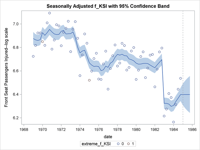
The following statements use the for1 data set to produce a time series plot of the seasonally adjusted f_KSI that highlights the additive outliers:

 proc sgplot data=for1;
    title "Seasonally Adjusted f_KSI with 95% Confidence Band";
    band x=date lower=smoothed_lower_f_KSI_sa 
       upper=smoothed_upper_f_KSI_sa ;
    series x=date y=smoothed_f_KSI_sa;
    refline '1jan1985'd / axis=x lineattrs=(pattern=shortdash)
       LEGENDLABEL= "Start of Multi-Step Forecasts" 
       name="Forecast Reference Line";
    scatter x=date y=f_KSI /group=extreme_f_KSI;
 run;

The generated plot is shown in Figure 27.9.

Figure 27.9 Plot of Seasonally Adjusted f_KSI that Highlights the Additive Outliers

The output data set, for1, also contains one-step-ahead residuals for f_KSI and r_KSI. You can use them for a variety of model diagnostic checks. For example, you can check the normality of the residuals by inspecting the residual-histogram. The following statements produce a residual-histogram for f_KSI:

 proc sgplot data=for1;
    title "Residual Histogram for f_KSI: Normality Check";
    histogram residual_f_KSI;
    density residual_f_KSI/type=normal;
    density residual_f_KSI/type=kernel;
 run;

Figure 27.10 shows the generated histogram along with the normal and kernel density estimates. It does not show any significant violation of the normality assumption.

Figure 27.10 Residual Histogram for f_KSI

Note: This procedure is experimental.