The PANEL Procedure
- Overview
-
Getting Started

-
Syntax
-
Details
Missing Values Computational Resources Restricted Estimates Notation The One-Way Fixed-Effects Model The Two-Way Fixed-Effects Model Balanced Panels Unbalanced Panels Between Estimators Pooled Estimator The One-Way Random-Effects Model The Two-Way Random-Effects Model Parks Method (Autoregressive Model) Da Silva Method (Variance-Component Moving Average Model) Dynamic Panel Estimator Linear Hypothesis Testing Heteroscedasticity-Corrected Covariance Matrices R Square Specification Tests Troubleshooting ODS Graphics The OUTPUT OUT= Data Set The OUTEST= Data Set The OUTTRANS= Data Set Printed Output ODS Table Names
-
Examples
- References
Example 20.2 The Airline Cost Data: Fixtwo Model
The Christenson Associates airline data are a frequently cited data set (see Greene 2000). The data measure costs, prices of inputs, and utilization rates for six airlines over the time span 1970–1984. This example analyzes the log transformations of the cost, price and quantity, and the raw (not logged) capacity utilization measure. You speculate the following model:
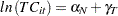 |
 |
 |
|||
 |
|
 |
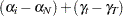
where the  are the pure cross-sectional effects and
  are the time effects. The actual model speculated is highly nonlinear in the original variables. It would look like the following:
 |
The data and preliminary SAS statements are:
data airline;
  input  Obs I T C Q PF LF;
  label obs = "Observation number";
  label I  = "Firm Number (CSID)";
  label T  = "Time period (TSID)";
  label Q  = "Output in revenue passenger miles (index)";
  label C  = "Total cost, in thousands";
  label PF = "Fuel price";
  label LF = "Load Factor (utilization index)";
datalines;

   ... more lines ...
data airline;
   set airline;
   lC = log(C);
   lQ = log(Q);
   lPF = log(PF);
   label lC = "Log transformation of costs";
   label lQ = "Log transformation of quantity";
   label lPF= "Log transformation of price of fuel";
run;
The following statements fit the model.
proc panel data=airline;
   id i t;
   model lC = lQ lPF LF / fixtwo;
run;
First, you see the model’s description in Output 20.2.1. The model is a two-way fixed-effects model. There are six cross sections and fifteen time observations.
| Model Description | |
|---|---|
| Estimation Method | FixTwo |
| Number of Cross Sections | 6 |
| Time Series Length | 15 |
The R square and degrees of freedom can be seen in Output 20.2.2. On the whole, you see a large R square, so there is a reasonable fit. The degrees of freedom of the estimate are 90 minus 14 time dummy variables minus 5 cross section dummy variables and 4 regressors.
| Fit Statistics | |||
|---|---|---|---|
| SSE | 0.1768 | DFE | 67 |
| MSE | 0.0026 | Root MSE | 0.0514 |
| R-Square | 0.9984 | ||
The F test for fixed effects is shown in Output 20.2.3. Testing the hypothesis that there are no fixed effects, you easily reject the null of poolability. There are group effects, or time effects, or both. The test is highly significant. OLS would not give reasonable results.
| F Test for No Fixed Effects | |||
|---|---|---|---|
| Num DF | Den DF | F Value | Pr > F |
| 19 | 67 | 23.10 | <.0001 |
Looking at the parameters, you see a more complicated pattern. Most of the cross-sectional effects are highly significant (with the exception of CS2). This means that the cross sections are significantly different from the sixth cross section. Many of the time effects show significance, but this is not uniform. It looks like the significance might be driven by a large  period effect, since the first six time effects are negative and of similar magnitude. The time dummy variables taper off in size and lose significance from time period 12 onward. There are many causes to which you could attribute this decay of time effects. The time period of the data spans the OPEC oil embargoes and the dissolution of the Civil Aeronautics Board (CAB). These two forces are two possible reasons to observe the decay and parameter instability. As for the regression parameters, you see that quantity affects cost positively, and the price of fuel has a positive effect, but load factors negatively affect the costs of the airlines in this sample. The somewhat disturbing result is that the fuel cost is not significant. If the time effects are proxies for the effect of the oil embargoes, then an insignificant fuel cost parameter would make some sense. If the dummy variables proxy for the dissolution of the CAB, then the effect of load factors is also not being precisely estimated.
| Parameter Estimates | ||||||
|---|---|---|---|---|---|---|
| Variable | DF | Estimate | Standard Error | t Value | Pr > |t| | Label |
| CS1 | 1 | 0.174237 | 0.0861 | 2.02 | 0.0470 | Cross Sectional Effect 1 |
| CS2 | 1 | 0.111412 | 0.0780 | 1.43 | 0.1576 | Cross Sectional Effect 2 |
| CS3 | 1 | -0.14354 | 0.0519 | -2.77 | 0.0073 | Cross Sectional Effect 3 |
| CS4 | 1 | 0.18019 | 0.0321 | 5.61 | <.0001 | Cross Sectional Effect 4 |
| CS5 | 1 | -0.04671 | 0.0225 | -2.08 | 0.0415 | Cross Sectional Effect 5 |
| TS1 | 1 | -0.69286 | 0.3378 | -2.05 | 0.0442 | Time Series Effect 1 |
| TS2 | 1 | -0.63816 | 0.3321 | -1.92 | 0.0589 | Time Series Effect 2 |
| TS3 | 1 | -0.59554 | 0.3294 | -1.81 | 0.0751 | Time Series Effect 3 |
| TS4 | 1 | -0.54192 | 0.3189 | -1.70 | 0.0939 | Time Series Effect 4 |
| TS5 | 1 | -0.47288 | 0.2319 | -2.04 | 0.0454 | Time Series Effect 5 |
| TS6 | 1 | -0.42705 | 0.1884 | -2.27 | 0.0267 | Time Series Effect 6 |
| TS7 | 1 | -0.39586 | 0.1733 | -2.28 | 0.0255 | Time Series Effect 7 |
| TS8 | 1 | -0.33972 | 0.1501 | -2.26 | 0.0269 | Time Series Effect 8 |
| TS9 | 1 | -0.2718 | 0.1348 | -2.02 | 0.0478 | Time Series Effect 9 |
| TS10 | 1 | -0.22734 | 0.0763 | -2.98 | 0.0040 | Time Series Effect 10 |
| TS11 | 1 | -0.1118 | 0.0319 | -3.50 | 0.0008 | Time Series Effect 11 |
| TS12 | 1 | -0.03366 | 0.0429 | -0.78 | 0.4354 | Time Series Effect 12 |
| TS13 | 1 | -0.01775 | 0.0363 | -0.49 | 0.6261 | Time Series Effect 13 |
| TS14 | 1 | -0.01865 | 0.0305 | -0.61 | 0.5430 | Time Series Effect 14 |
| Intercept | 1 | 12.93834 | 2.2181 | 5.83 | <.0001 | Intercept |
| lQ | 1 | 0.817264 | 0.0318 | 25.66 | <.0001 | Log transformation of quantity |
| lPF | 1 | 0.168732 | 0.1635 | 1.03 | 0.3057 | Log transformation of price of fuel |
| LF | 1 | -0.88267 | 0.2617 | -3.37 | 0.0012 | Load Factor (utilization index) |