The PANEL Procedure
- Overview
-
Getting Started

-
Syntax
-
Details
Missing Values Computational Resources Restricted Estimates Notation The One-Way Fixed-Effects Model The Two-Way Fixed-Effects Model Balanced Panels Unbalanced Panels Between Estimators Pooled Estimator The One-Way Random-Effects Model The Two-Way Random-Effects Model Parks Method (Autoregressive Model) Da Silva Method (Variance-Component Moving Average Model) Dynamic Panel Estimator Linear Hypothesis Testing Heteroscedasticity-Corrected Covariance Matrices R Square Specification Tests Troubleshooting ODS Graphics The OUTPUT OUT= Data Set The OUTEST= Data Set The OUTTRANS= Data Set Printed Output ODS Table Names
-
Examples
- References
| Da Silva Method (Variance-Component Moving Average Model) |
The Da Silva method assumes that the observed value of the dependent variable at the tth time point on the ith cross-sectional unit can be expressed as
 |
where
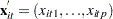 is a vector of explanatory variables for the tth time point and ith cross-sectional unit
 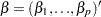 is the vector of parameters
  is a time-invariant, cross-sectional unit effect
  is a cross-sectionally invariant time effect
  is a residual effect unaccounted for by the explanatory variables and the specific time and cross-sectional unit effects
Since the observations are arranged first by cross sections, then by time periods within cross sections, these equations can be written in matrix notation as
 |
where
 |
 |
 |
 |
 |
 |
Here 1  is an
is an  vector with all elements equal to 1, and
  denotes the Kronecker product.
The following conditions are assumed:
 is a sequence of nonstochastic, known
  vectors in
  whose elements are uniformly bounded in . The matrix X has a full column rank p.
  is a
is a  constant vector of unknown parameters.
 a is a vector of uncorrelated random variables such that
 and
and  ,
,  .
. b is a vector of uncorrelated random variables such that
 and
and  where
where  and
and  .
. -
 is a sample of a realization of a finite moving-average time series of order
  for each i ; hence,
where
 are unknown constants such that
  and
and  , and
, and  is a white noise process—that is, a sequence of uncorrelated random variables with
  , and
, and  .
. The sets of random variables
 ,
,  , and
, and  for
for  are mutually uncorrelated.
 The random terms have normal distributions
 and
and  for
for  and
and  .
.
If assumptions 1–6 are satisfied, then
 |
and
 |
where  is a
is a  matrix with elements
  as follows:
 |
where 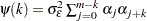 for
for  . For the definition of
  ,
,  ,
,  , and
, and  , see the section Fuller and Battese’s Method.
The covariance matrix, denoted by V, can be written in the form
 |
where  , and, for k =1,
 , m,
, m,  is a band matrix whose kth off-diagonal elements are 1’s and all other elements are 0’s.
Thus, the covariance matrix of the vector of observations y has the form
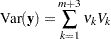 |
where
 |
 |
 |
|||
 |
|
 |
|||
 |
|
 |
|||
 |
|
 |
|||
 |
|
 |
|||
 |
|
 |
The estimator of is a two-step GLS-type estimator—that is, GLS with the unknown covariance matrix replaced by a suitable estimator of V. It is obtained by substituting Seely estimates for the scalar multiples  .
.
Seely (1969) presents a general theory of unbiased estimation when the choice of estimators is restricted to finite dimensional vector spaces, with a special emphasis on quadratic estimation of functions of the form  .
.
The parameters  (i =1,, n) are associated with a linear model E(y )=X
  with covariance matrix
  where
where  (i =1, , n) are real symmetric matrices. The method is also discussed by Seely (1970a,1970b) and Seely and Zyskind (1971). Seely and Soong (1971) consider the MINQUE principle, using an approach along the lines of Seely (1969).