The PANEL Procedure

The HCCME= option in the MODEL statement selects the type of heteroscedasticity-consistent covariance matrix. In the presence of heteroscedasticity, the covariance matrix has a complicated structure which can result in inefficiencies in the OLS estimates and biased estimates of the variance covariance matrix. Consider the simple linear model:

This discussion parallels the discussion in Davidson and MacKinnon, 1993, pg. 548–562. The assumptions that make the linear regression best linear unbiased estimator (BLUE) are and , where has the simple structure . Heteroscedasticity results in a general covariance structure, so that it is not possible to simplify . The result is the following:

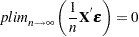
As long as the following is true, then you are assured that the OLS estimate is consistent and unbiased:

If the regressors are nonrandom, then it is possible to write the variance of the estimated as the following:

The effect of structure in the variance-covariance matrix can be ameliorated by using generalized least squares (GLS), provided that can be calculated. Using , you premultiply both sides of the regression equation,

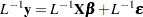where denotes the Cholesky root of . (that is, with lower triangular).

The resulting GLS is

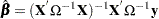Using the GLS , you can write

The resulting variance expression for the GLS estimator is

The difference in variance between the OLS estimator and the GLS estimator can be written as

By the Gauss-Markov theorem, the difference matrix must be positive definite under most circumstances (zero if OLS and GLS are the same, when the usual classical regression assumptions are met). Thus, OLS is not efficient under a general error structure. It is crucial to realize that OLS does not produce biased results. It would suffice if you had a method for estimating a consistent covariance matrix and you used the OLS . Estimation of the matrix is certainly not simple. The matrix is square and has elements; unless some sort of structure is assumed, it becomes an impossible problem to solve. However, the heteroscedasticity can have quite a general structure. White (1980) shows that it is not necessary to have a consistent estimate of . On the contrary, it suffices to calculate an estimate of the middle expression. That is, you need an estimate of:

This matrix, , is easier to estimate because its dimension is K. PROC PANEL provides the following classical HCCME estimators for :

The matrix is approximated by:

• HCCME=N0:

  This is the simple OLS estimator. If you do not specify the HCCME= option, PROC PANEL defaults to this estimator.

• HCCME=0:

  where is the number of cross sections and is the number of observations in th cross section. The is from the th observation in the th cross section, constituting the th row of the matrix . If the CLUSTER option is specified, one extra term is added to the preceding equation so that the estimator of matrix is

• HCCME=1:

  where is the total number of observations, , and is the number of parameters. With the CLUSTER option, the estimator becomes

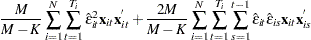
• HCCME=2:

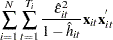
  The term is the th diagonal element of the hat matrix. The expression for is . The hat matrix attempts to adjust the estimates for the presence of influence or leverage points. With the CLUSTER option, the estimator becomes

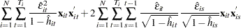
• HCCME=3:

  With the CLUSTER option, the estimator becomes

• HCCME=4: PROC PANEL includes this option for the calculation of the Arellano (1987) version of the White (1980) HCCME in the panel setting. Arellano’s insight is that there are covariance matrices in a panel, and each matrix corresponds to a cross section. Forming the White HCCME for each panel, you need to take only the average of those estimators that yield Arellano. The details of the estimation follow. First, you arrange the data such that the first cross section occupies the first observations. You treat the panels as separate regressions with the form:

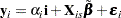
  The parameter estimates and are the result of least squares dummy variables (LSDV) or within estimator regressions, and is a vector of ones of length . The estimate of the th cross section’s matrix (where the subscript indicates that no constant column has been suppressed to avoid confusion) is . The estimate for the whole sample is:

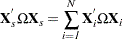
  The Arellano standard error is in fact a White-Newey-West estimator with constant and equal weight on each component. In the between estimators, selecting HCCME=4 returns the HCCME=0 result since there is no 'other' variable to group by.

In their discussion, Davidson and MacKinnon (1993, pg. 554) argue that HCCME=1 should always be preferred to HCCME=0. Although HCCME=3 is generally preferred to 2 and 2 is preferred to 1, the calculation of HCCME=1 is as simple as the calculation of HCCME=0. Therefore, it is clear that HCCME=1 is preferred when the calculation of the hat matrix is too tedious.

All HCCME estimators have well-defined asymptotic properties. The small sample properties are not well-known, and care must exercised when sample sizes are small.

The HCCME estimator of is used to drive the covariance matrices for the fixed effects and the Lagrange multiplier standard errors. Robust estimates of the variance-covariance matrix for imply robust variance-covariance matrices for all other parameters.